Working with linear regression is a sometimes under-appreciated trait in data science. As a generalization of very fundamental statistical concepts like t-tests and analysis of variance it has deep ties into the realm of statistics, and can serve as a powerful tool to explain variance in data. Since linear models are only linear in their parameters, they can also describe polynomial and even multiplicative relationships.
But due to parametric nature, linear regression is also more vulnerable to extreme values and multicollinearity in the data, of which we want to analyze the latter in more detail, using a simulation. Among many other issues, multicollinearity may produce non-robust models (staggering coefficients) and may undermine statistical significance.
Before we run our simulations we will look into the impact of multicollinearity on a simple linear model. We will use a data set from Stat Trek which contains test scores and some other performance measures (like IQ or GPA) of students:
# wrap in function to ensure immutability of raw data
get_test_score_data <- function() {
  # data from https://stattrek.com/multiple-regression/multicollinearity.aspx
  dplyr::tibble(test_score = c(100, 95, 92, 90, 85, 80, 78, 75, 72, 65),
                iq = c(125, 104, 110, 105, 100, 100, 95, 95, 85, 90),
                study_hours = c(30, 40, 25, 20, 20, 20, 15, 10, 0, 5),
                gpa = c(3.9, 2.6, 2.7, 3, 2.4, 2.2, 2.1, 2.1, 1.5, 1.8))
}

data <- get_test_score_data()
## # A tibble: 10 × 4
##    test_score    iq study_hours   gpa
##         <dbl> <dbl>       <dbl> <dbl>
##  1        100   125          30   3.9
##  2         95   104          40   2.6
##  3         92   110          25   2.7
##  4         90   105          20   3
##  5         85   100          20   2.4
##  6         80   100          20   2.2
##  7         78    95          15   2.1
##  8         75    95          10   2.1
##  9         72    85           0   1.5
## 10         65    90           5   1.8
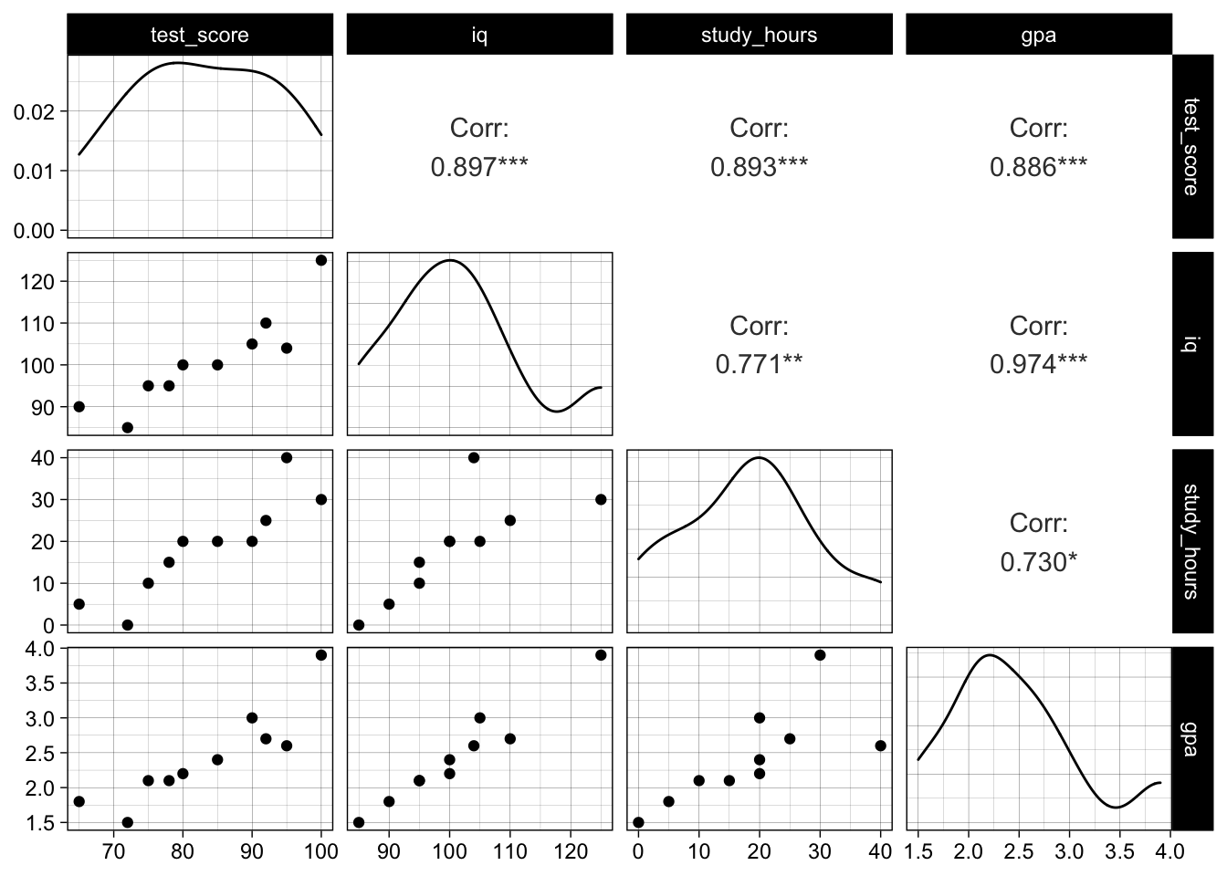
We observe a high correlation between all variables, and especially iq and gpa are very strongly correlated:
GGally::ggpairs(data)
If we fit a simple model to explain the test score using iq and study_hours we can see that their effect is statistically significant (p-values around 0.03 and overall significance):
simple_model <- lm(test_score ~ iq + study_hours, data = data)
sqrt(mean((simple_model$residuals)^2))
## [1] 3.242157
summary(simple_model)
##
## Call:
## lm(formula = test_score ~ iq + study_hours, data = data)
##
## Residuals:
##    Min     1Q Median     3Q    Max
## -6.341 -1.130 -0.191  1.450  5.542
##
## Coefficients:
##             Estimate Std. Error t value Pr(>|t|)
## (Intercept)  23.1561    15.9672   1.450   0.1903
## iq            0.5094     0.1808   2.818   0.0259 *
## study_hours   0.4671     0.1720   2.717   0.0299 *
## ---
## Signif. codes:  0 '***' 0.001 '**' 0.01 '*' 0.05 '.' 0.1 ' ' 1
##
## Residual standard error: 3.875 on 7 degrees of freedom
## Multiple R-squared:  0.9053,	Adjusted R-squared:  0.8782
## F-statistic: 33.45 on 2 and 7 DF,  p-value: 0.0002617
If we add gpa to the model, we expectedly receive a smaller (in-sample) error, but severely different estimates for intercept and slopes. Also, iq and gpa are not significant any more. This is due to their collinearity and well described here.
# estimates and p values very different
full_model <- lm(test_score ~ iq + study_hours + gpa, data = data)
sqrt(mean((full_model$residuals)^2))
## [1] 3.061232
summary(full_model)
##
## Call:
## lm(formula = test_score ~ iq + study_hours + gpa, data = data)
##
## Residuals:
##     Min      1Q  Median      3Q     Max
## -6.3146 -1.2184 -0.4266  1.5516  5.6358
##
## Coefficients:
##             Estimate Std. Error t value Pr(>|t|)
## (Intercept) 50.30669   35.70317   1.409   0.2085
## iq           0.05875    0.55872   0.105   0.9197
## study_hours  0.48876    0.17719   2.758   0.0329 *
## gpa          7.37578    8.63161   0.855   0.4256
## ---
## Signif. codes:  0 '***' 0.001 '**' 0.01 '*' 0.05 '.' 0.1 ' ' 1
##
## Residual standard error: 3.952 on 6 degrees of freedom
## Multiple R-squared:  0.9155,	Adjusted R-squared:  0.8733
## F-statistic: 21.68 on 3 and 6 DF,  p-value: 0.001275
BIC(full_model, simple_model)
##              df      BIC
## full_model    5 62.26804
## simple_model  4 61.11389
In a normal prediction modeling scenario we would try to avoid this situation by using regularization to automate the feature selection, and therefore improve the generalization power and robustness of our model while keeping up good predictability at the same time. In classical statistics we do not only care for predictability (low error) but also statistical significance of variables (p-values) and causality.
A traditional approach here is to use variance inflation factors to remove variables from the equation. Instead of looking at only pairwise correlation of predictors we try to look at linear dependence of the predictors: we essentially try to estimate one predictor by all other predictors, the variance inflation factor is then given as an inverse of the unexplained variance (i.e.1 / (1 - R.sq.)). This value will be high if the predictor can be linearly represented by the others, and low if not. As a rule of thumb, if it is above 4 the predictor should potentially be dropped.
vif_gpa_model <- lm(gpa ~ iq + study_hours, data = data)
vif_gpa_factor <- 1 / (1 - summary(vif_gpa_model)$r.squared)
vif_gpa_factor
## [1] 19.65826
We can easily do this for all predictors and decide to drop features with high inflation factors.
car::vif(full_model)
##          iq study_hours         gpa
##   22.643553    2.517786   19.658264
Domain knowledge may tell us that GPA is rather a result of IQ than vice versa, therefore adding IQ as an independent variable might be more reasonable than using the proxy variable GPA.
Simulation 1: running “many models” with purrr 🔗
To get a feel for the harming effect of multicollinearity in the data let us simulate what may happen to our model coefficients when we fit a linear regression with different features repeatedly.
To do this we will use purrr, which helps us to run our own functions in a vectorized fashion on top of lists of dataframes, and therefore over data and/or models (recommended reads: in R for Data Science but also official documentation and cheat sheets of purrr).
To understand our simulation, let us first simulate drawing some dummy data from a simple linear relation y = 5 + 3 * x and fit a linear model multiple times. We create some helper functions to draw reproducible samples and fit models:
generate_dummy_data <- function(data, seed = NULL) {
  set.seed(seed = seed)
  data <- dplyr::tibble(x = rnorm(100, 50, 10),
                        y = 5 + 3 * x + rnorm(100, 0, 0.1))
  return(data)
}

generate_dummy_model <- function(data) {
  model <- lm(y ~ x, data = data)
  return(model)
}
We can now run this simulation multiple times and extract the model coefficients (intercept & slope) using purrr::map:
extract_model_coefficients <- function(model) {
  coefs <- broom::tidy(model)
  # replace dots and white spaces with underscores
  colnames(coefs) <- gsub(pattern = "\\.| ",
                          replacement = "_",
                          x = colnames(coefs))
  return(coefs)
}

run_lm_simulation <- function(data_generator, model_generator, n = 1000) {
  simulation <-
    dplyr::tibble(i = 1:n) %>%
    dplyr::mutate(
      data = purrr::map(.x = i, .f = ~ data_generator(seed = .x)),
      model = purrr::map(.x = data, .f = model_generator),
      coefs = purrr::map(.x = model, .f = extract_model_coefficients)
      ) %>%
  return(simulation)
}
dummy_simulation <- run_lm_simulation(data_generator = generate_dummy_data,
                                      model_generator = generate_dummy_model,
                                      n = 1000)
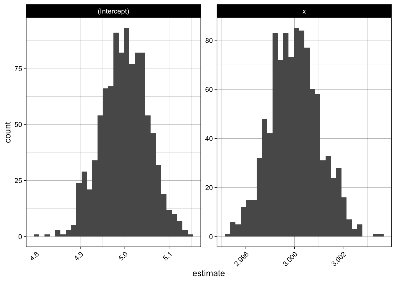
We see that the estimates are very stable and close to the true values.
dummy_simulation %>%
  tidyr::unnest(coefs) %>%
  ggplot(aes(x = estimate)) +
  geom_histogram(bins = 30) +
  facet_wrap(~ term, scales = "free") +
  theme(axis.text.x = element_text(angle = 45, hjust = 1))
Now let us apply this to our test score data, by using bootstrapped samples:
generate_data <- function(size = 30, seed = NULL) {
  data <- get_test_score_data()

  # bootstrap sample
  sampled_data <- data[sample(1:nrow(data), size = size, replace = TRUE), ]

  # add some noise to mitigate obvious clusters in the data
  sampled_data <-
    sampled_data %>%
    dplyr::mutate(
      test_score = test_score + round(rnorm(size, mean = 0, sd = 1)),
      iq = iq + round(rnorm(size, mean = 0, sd = 1)),
      study_hours = study_hours + round(rnorm(size, mean = 0, sd = 1)),
      gpa = gpa + rnorm(size, mean = 1, sd = 0.1)
      )

  # rescale gpa to range between 0 and 4
  sampled_data <- sampled_data %>% dplyr::mutate(gpa = gpa / max(gpa) * 4)
  return(sampled_data)
}
We will not only look at one model, but compare two models: the full model using all features (i.e. suffering from multicollinearity) and one using a reduced set of features:
generate_full_model <- function(data) {
  model <- lm(test_score ~ iq + study_hours + gpa, data = data)
  return(model)
}

generate_simple_model <- function(data) {
  model <- lm(test_score ~ iq + study_hours, data = data)
  return(model)
}

full_model_simulations <- run_lm_simulation(data_generator = generate_data,
                                            model_generator = generate_full_model)
simple_model_simulations <- run_lm_simulation(data_generator = generate_data,
                                              model_generator = generate_simple_model)

simulations <- dplyr::bind_rows(full = full_model_simulations,
                                simple = simple_model_simulations,
                                .id = "name")
head(simulations)
## # A tibble: 6 × 5
##   name      i data              model  coefs
##   <chr> <int> <list>            <list> <list>
## 1 full      1 <tibble [30 × 4]> <lm>   <tibble [4 × 5]>
## 2 full      2 <tibble [30 × 4]> <lm>   <tibble [4 × 5]>
## 3 full      3 <tibble [30 × 4]> <lm>   <tibble [4 × 5]>
## 4 full      4 <tibble [30 × 4]> <lm>   <tibble [4 × 5]>
## 5 full      5 <tibble [30 × 4]> <lm>   <tibble [4 × 5]>
## 6 full      6 <tibble [30 × 4]> <lm>   <tibble [4 × 5]>
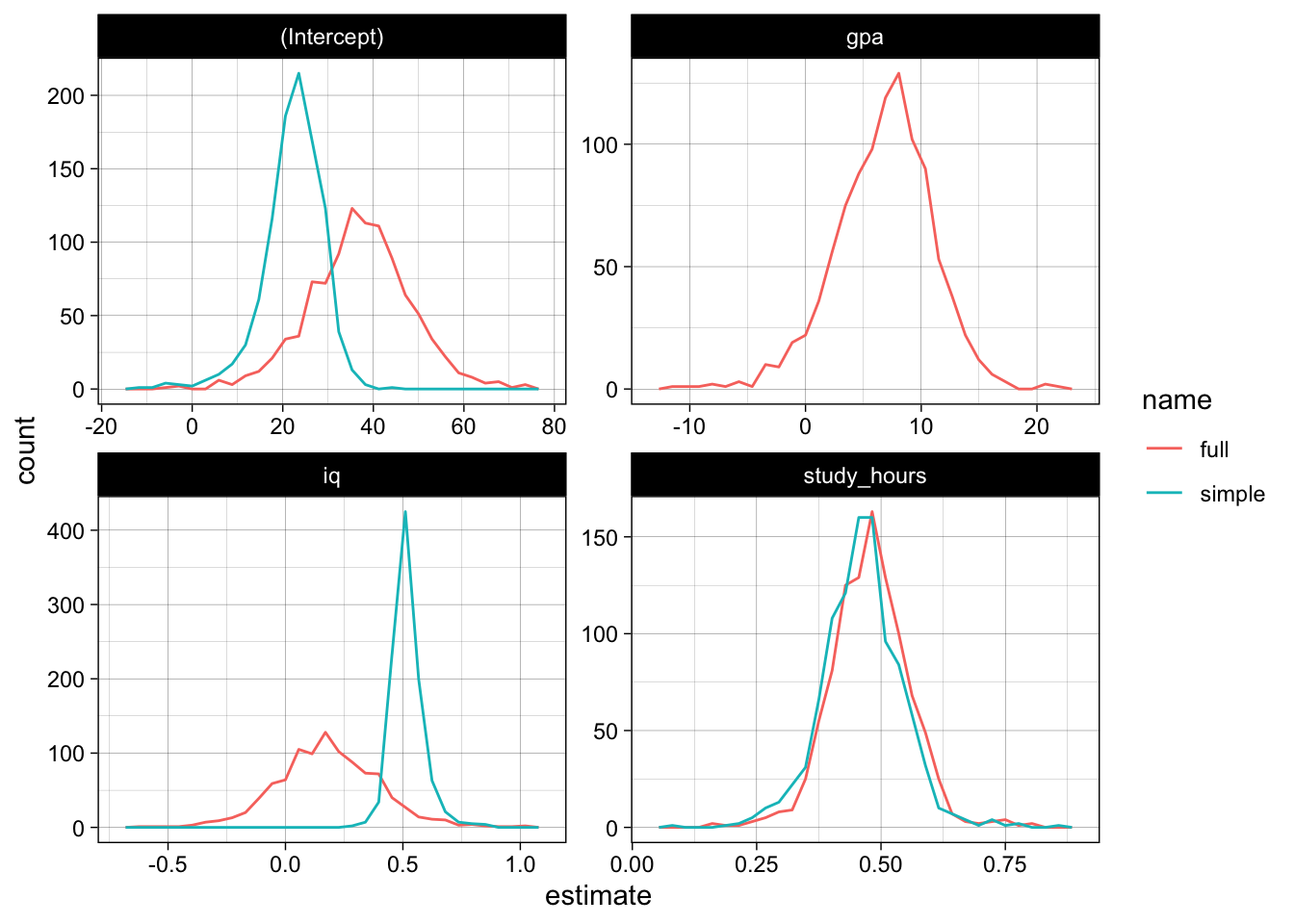
Let us plot the estimates for intercept and slopes in both models (using ggplot2 and theme_set(theme_linedraw())). We see a huge difference in the intercept, but also for the iq-coefficient:
model_coefs <-
  simulations %>%
  dplyr::select(name, coefs) %>%
  tidyr::unnest(coefs)

model_coefs %>%
  ggplot(aes(x = estimate, color = name)) +
  geom_freqpoly(bins = 30) +
  facet_wrap( ~ term, scales = "free")
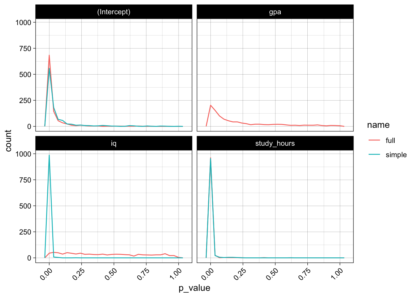
The p-values also do not look really promising, the model has trouble gaining confidence about the relevance of iq and gpa, the p-values do not really concentrate at the lower end:
model_coefs %>%
  ggplot(aes(x = p_value, color = name)) +
  geom_freqpoly(bins = 30) +
  facet_wrap( ~ term) +
  theme(axis.text.x = element_text(angle = 45, hjust = 1))
Simulation 2: parallel model evaluation 🔗
Let us run another simulation on a slightly bigger dataset, where we additionally compute some test data error metric.
We will perform simulation in a slightly different way: We will evaluate the different models in parallel, and since we are only interested in the coefficient estimates and the error metrics we will avoid transferring too much data from the workers and not store training data and model objects itself.
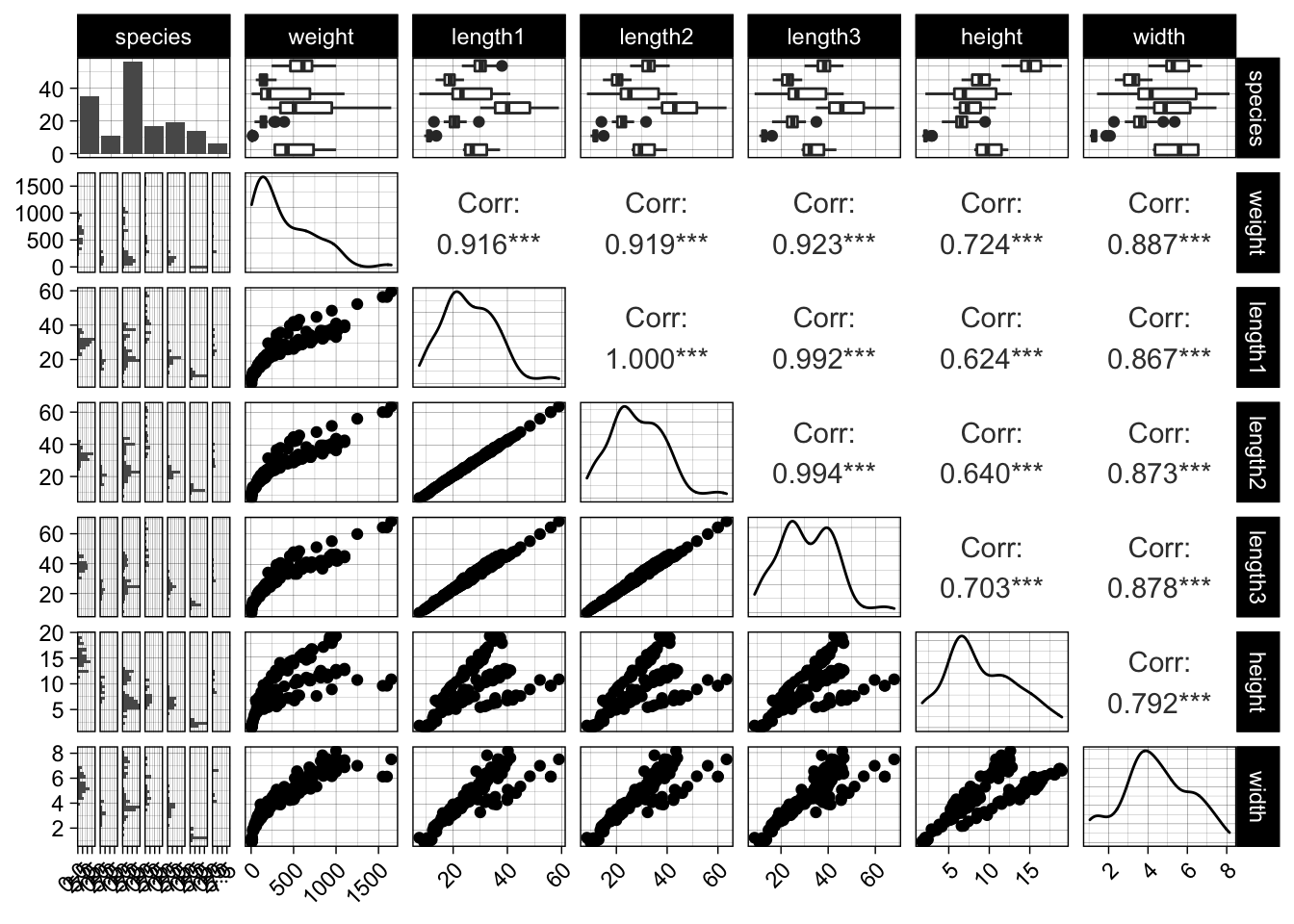
Let us look at the fishmarket dataset, which consists of different fish measurements (length, width, height) of different species and their weight. The measurements are again highly correlated. We will try to predict the weight and also use some naive domain knowledge in the process. Let us remove some obvious outliers, i.e. measurement errors.
url <- "https://tinyurl.com/fish-market-dataset"
raw_data <- readr::read_csv(url)
## Rows: 159 Columns: 7
## ── Column specification ────────────────────────────────────────────────────────
## Delimiter: ","
## chr (1): Species
## dbl (6): Weight, Length1, Length2, Length3, Height, Width
##
## ℹ Use `spec()` to retrieve the full column specification for this data.
## ℹ Specify the column types or set `show_col_types = FALSE` to quiet this message.
data <-
  raw_data %>%
  dplyr::rename_all(tolower) %>%
  dplyr::mutate(species = tolower(species)) %>%
  dplyr::filter(weight > 0)

dplyr::sample_n(data, 5)
## # A tibble: 5 × 7
##   species   weight length1 length2 length3 height width
##   <chr>      <dbl>   <dbl>   <dbl>   <dbl>  <dbl> <dbl>
## 1 bream        950    38      41      46.5   17.6  6.37
## 2 bream        390    27.6    30      35     12.7  4.69
## 3 whitefish    800    33.7    36.4    39.6   11.8  6.57
## 4 bream        650    31      33.5    38.7   14.5  5.73
## 5 perch        690    34.6    37      39.3   10.6  6.37
GGally::ggpairs(data) +
  theme(axis.text.x = element_text(angle = 45, hjust = 1))
## `stat_bin()` using `bins = 30`. Pick better value with `binwidth`.
## `stat_bin()` using `bins = 30`. Pick better value with `binwidth`.
## `stat_bin()` using `bins = 30`. Pick better value with `binwidth`.
## `stat_bin()` using `bins = 30`. Pick better value with `binwidth`.
## `stat_bin()` using `bins = 30`. Pick better value with `binwidth`.
## `stat_bin()` using `bins = 30`. Pick better value with `binwidth`.
data %>%
  ggplot(aes(x = length1, y = weight)) +
  geom_point() +
  geom_smooth(method = "loess")
## `geom_smooth()` using formula 'y ~ x'
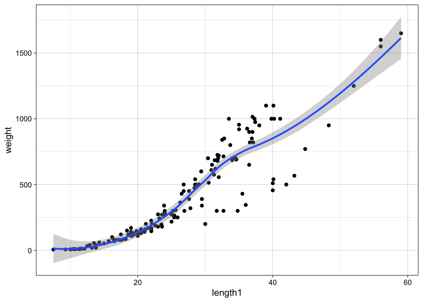
As weight is somewhat proportional to volume we can probably find a relationship like weight ~ length^3, therefore we can fit log(weight) ~ log(length) which will lead to estimates a, b for log(weight) ~ a + b * log(length). Therefore, after exponentiation weight ~ exp(a) * length^b, where we would expect b around 3, and a some scaling factor:
simple_log_log_model <- lm(log(weight) ~ log(length1), data = data)
summary(simple_log_log_model)
##
## Call:
## lm(formula = log(weight) ~ log(length1), data = data)
##
## Residuals:
##      Min       1Q   Median       3Q      Max
## -0.90870 -0.07280  0.07773  0.26639  0.50636
##
## Coefficients:
##              Estimate Std. Error t value Pr(>|t|)
## (Intercept)  -4.62769    0.23481  -19.71   <2e-16 ***
## log(length1)  3.14394    0.07296   43.09   <2e-16 ***
## ---
## Signif. codes:  0 '***' 0.001 '**' 0.01 '*' 0.05 '.' 0.1 ' ' 1
##
## Residual standard error: 0.3704 on 156 degrees of freedom
## Multiple R-squared:  0.9225,	Adjusted R-squared:  0.922
## F-statistic:  1857 on 1 and 156 DF,  p-value: < 2.2e-16
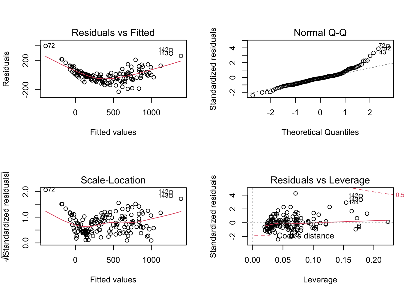
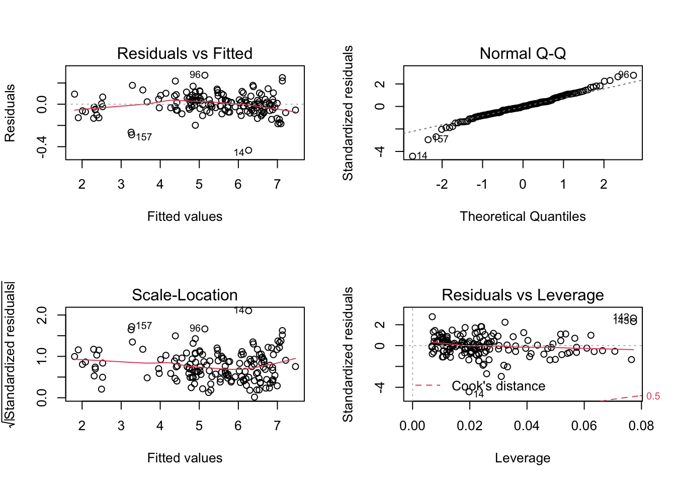
Fair enough, b is around 3.14. Adding height and width may increase the model performance again. Before we jump into it, let us quickly build another naive model without the log-transformations, to see the poor fit due to the nonlinear relationship and increasing variance by looking at the residual plots.
naive_model <- lm(weight ~ length1 + width + height + species, data = data)
par(mfrow=c(2,2))
plot(naive_model)
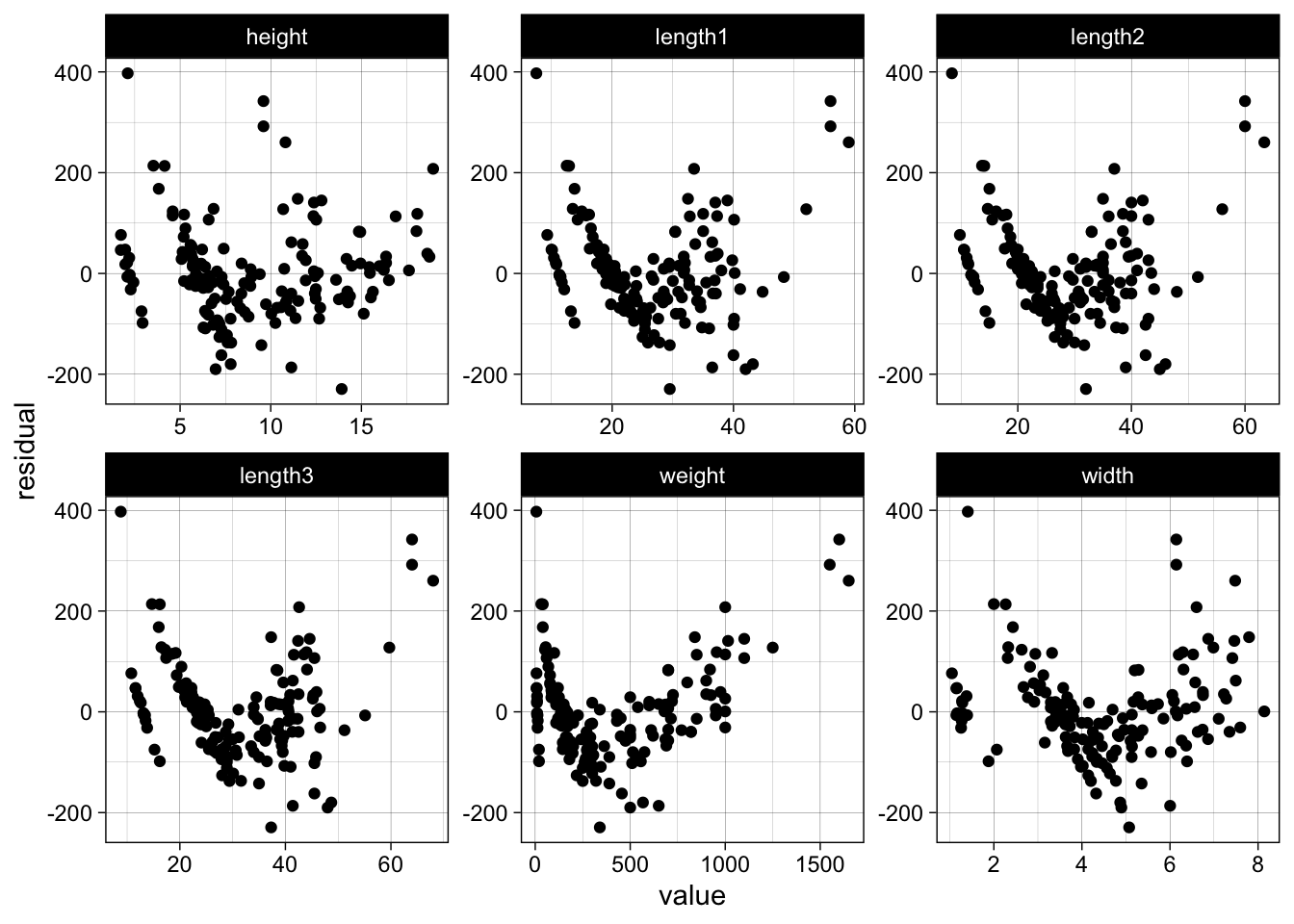
# plot residuals against all features
data %>%
  dplyr::mutate(residual = naive_model$residuals) %>%
  dplyr::select(-species) %>%
  # convert to wide to long for plotting
  tidyr::gather(key, value, -residual) %>%
  ggplot(aes(x = value, y = residual)) +
  geom_point() +
  facet_wrap(~ key, scales = "free")
Now back to the log-log model, which we assume will perform much better.
log_log_model <- lm(log(weight) ~ log(length1) + log(width) + log(height), data = data)

par(mfrow=c(2,2))
plot(log_log_model)
data %>%
  dplyr::mutate(residual = log_log_model$residuals) %>%
  dplyr::select(-species) %>%
  tidyr::gather(key, value, -residual) %>%
  ggplot(aes(x = value, y = residual)) +
  geom_point() +
  facet_wrap(~ key, scales = "free")
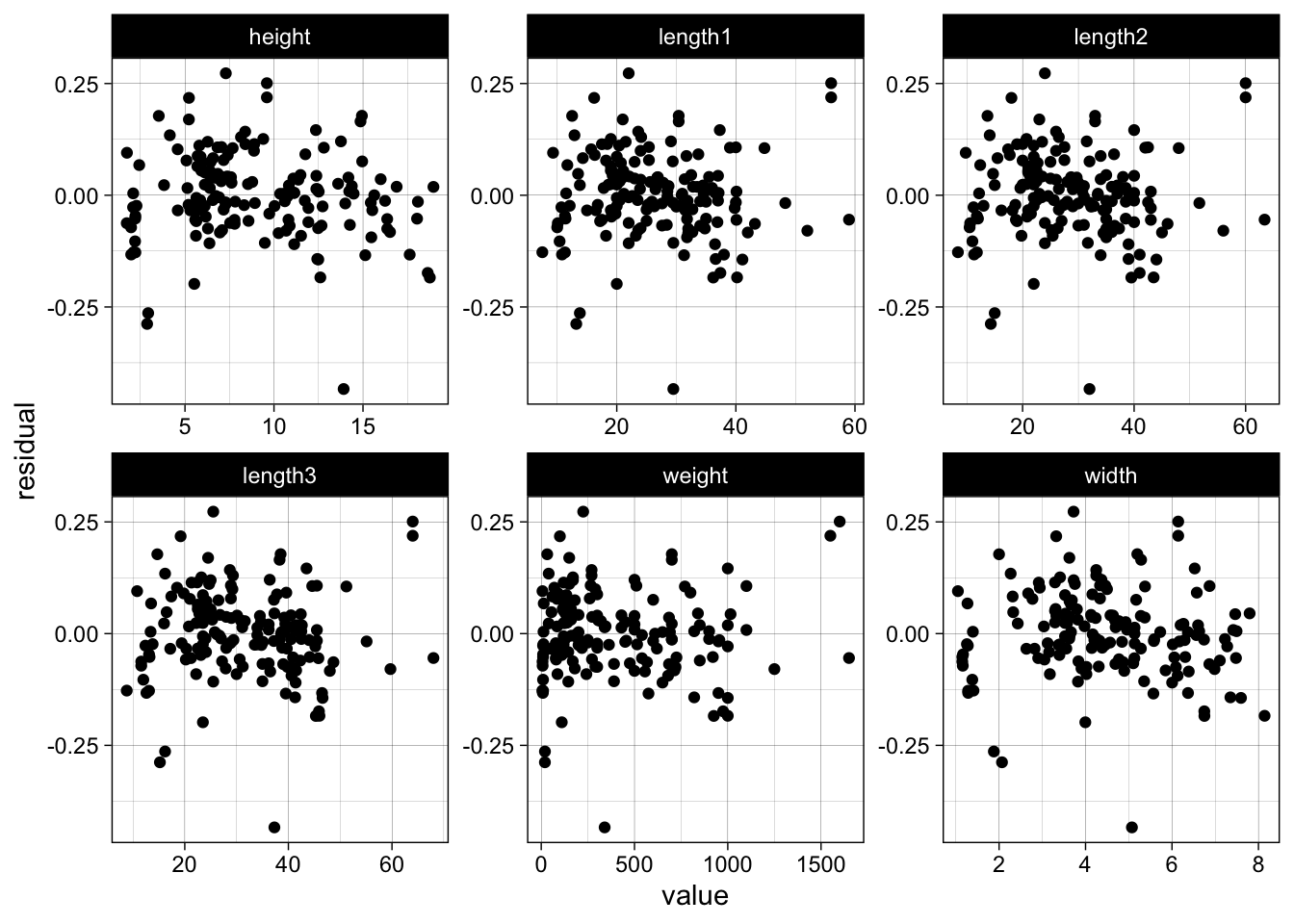
We see no trend or severe funnel effect in the residuals. In general a log-log model makes sense when we expect that a x% increase will lead to a y% increase in the response.
We use caret::dummyVars to one-hot encode our species feature (in lm we could also use factors, but those will not work with glmnet):
one_hot_encoder <- caret::dummyVars( ~ ., data = data)
data <- dplyr::as_tibble(predict(one_hot_encoder, newdata = data))
Instead of using R formulas we will actually log-transform our features:
numeric_features <- c("length1", "length2", "length3", "height", "width")

data <-
  data %>%
  dplyr::mutate_at(numeric_features, log) %>%
  dplyr::rename_at(numeric_features, function(x) paste0(x, "_log"))

x <- data %>% dplyr::select(-weight)
y <- data %>% dplyr::pull(weight)
generate_data <- function(seed=NULL, test_size=1/4) {
  n <- nrow(x)
  set.seed(seed)
  train_idx <- sample(1:n, size = (1-test_size) * n)

  return(list(x_train = x[train_idx,],
              x_test = x[-train_idx,],
              y_train = y[train_idx],
              y_test = y[-train_idx]))
}

head(generate_data(1)$x_train)
## # A tibble: 6 × 12
##   speciesbream speciesparkki speciesperch speciespike speciesroach speciessmelt
##          <dbl>         <dbl>        <dbl>       <dbl>        <dbl>        <dbl>
## 1            0             1            0           0            0            0
## 2            0             0            0           1            0            0
## 3            0             0            0           0            1            0
## 4            1             0            0           0            0            0
## 5            0             0            0           0            1            0
## 6            0             0            1           0            0            0
## # … with 6 more variables: specieswhitefish <dbl>, length1_log <dbl>,
## #   length2_log <dbl>, length3_log <dbl>, height_log <dbl>, width_log <dbl>
On top of normal linear models we will also fit regularized linear models (Ridge, Lasso and Elastic net), using the glmnet package. We create a wrapper function which we can use to pass a seed and a named list with model parameters. The function itself will then generate the data depending on the seed using the function defined above.
fit_glmnet <- function(seed=NULL, params=NULL) {
  data <- generate_data(seed)

  x_train <- data$x_train
  x_test <- data$x_test
  y_train <- data$y_train
  y_test <- data$y_test

  # pluck selects from named list and allows defaults if value is missing
  features <- purrr::pluck(params, "features", .default = colnames(x_train))
  lambda <- purrr::pluck(params, "lambda", .default = 0)
  alpha <- purrr::pluck(params, "alpha", .default = 0)

  x_train <- x_train[,features]
  x_test <- x_test[,features]

  # train log model
  model <- glmnet::glmnet(x = data.matrix(x_train),
                          y = log(y_train),
                          lambda = lambda,
                          alpha = alpha)

  log_predictions <- predict(object = model, newx = data.matrix(x_test))
  # transform back
  predictions <- exp(log_predictions)

  residuals <- y_test - predictions
  rmse <- sqrt(mean((residuals^2)))

  # extracting tidy glmnet coefs is a bit cumbersome..
  coefs_glmnet <- coef(model)
  coefs <- dplyr::tibble(term = rownames(coefs_glmnet),
                         estimate = matrix(coefs_glmnet)[,1])

  return(list(coefs = coefs,
              rmse = rmse))
}
Let us test our function with some parameters:
params <- list(features = c("length1_log", "height_log", "width_log"))
fit_glmnet(seed = 1, params = params)
## $coefs
## # A tibble: 4 × 2
##   term        estimate
##   <chr>          <dbl>
## 1 (Intercept)   -1.95
## 2 length1_log    1.50
## 3 height_log     0.652
## 4 width_log      0.876
##
## $rmse
## [1] 26.5608
Fitting again, with the same seed and params will produce the same estimates:
fit_glmnet(seed = 1, params = params)
## $coefs
## # A tibble: 4 × 2
##   term        estimate
##   <chr>          <dbl>
## 1 (Intercept)   -1.95
## 2 length1_log    1.50
## 3 height_log     0.652
## 4 width_log      0.876
##
## $rmse
## [1] 26.5608
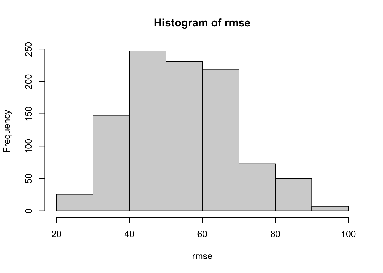
We can now easily run the simulation multiple times using purrr::map and extract the errors using purrr::map_dbl.
simulations <- purrr::map(1:1000, fit_glmnet)
rmse <- purrr::map_dbl(simulations, "rmse")
hist(rmse)
Let us run the simulation with different parameter combinations now. We will add our parameters to a dataframe, to be able to run the simulation rowwise and in parallel, both over models and seeds:
params <- list(ridge = list(lambda = 0.1, alpha = 0),
               lasso = list(lambda = 0.01, alpha = 1),
               elastic_net = list(lambda = 0.01, alpha = 0.5),
               full = list(lambda = 0),
               simple = list(features = c("length1_log", "width_log", "height_log"),
                             lambda = 0))

params_df <- dplyr::tibble(name=factor(names(params)),
                           params=params)

params_df
## # A tibble: 5 × 2
##   name        params
##   <fct>       <named list>
## 1 ridge       <named list [2]>
## 2 lasso       <named list [2]>
## 3 elastic_net <named list [2]>
## 4 full        <named list [1]>
## 5 simple      <named list [2]>
We will add and unnest the seeds now:
n_simulations <- 1000
n_workers <- 10

simulations <-
  params_df %>%
  dplyr::mutate(seed = list(1:n_simulations)) %>%
  tidyr::unnest(seed)

head(simulations)
## # A tibble: 6 × 3
##   name  params            seed
##   <fct> <named list>     <int>
## 1 ridge <named list [2]>     1
## 2 ridge <named list [2]>     2
## 3 ridge <named list [2]>     3
## 4 ridge <named list [2]>     4
## 5 ridge <named list [2]>     5
## 6 ridge <named list [2]>     6
Using this dataframe we can now run the simulations rowwise and in parallel
using furrr::future_map2 as the parallel version of purrr::map2.
We signal furrr that we have taken care of setting a seed by passing
furrr::furrr_options(seed = NULL) to the function call.
tictoc::tic()

future::plan(future::multisession, workers = n_workers)

simulations <-
  simulations %>%
  dplyr::mutate(
    simulation = furrr::future_map2(
      .x = seed,
      .y = params,
      .f = fit_glmnet,
      .options = furrr::furrr_options(seed = NULL)
      ),
    rmse = purrr::map_dbl(simulation, "rmse"),
    coefs = purrr::map(simulation, "coefs")
    )

tictoc::toc()
## 13.34 sec elapsed
Let us look at the distribution of our errors for the different models:
simulations %>%
  ggplot(aes(x = rmse, color = name)) +
  geom_boxplot()
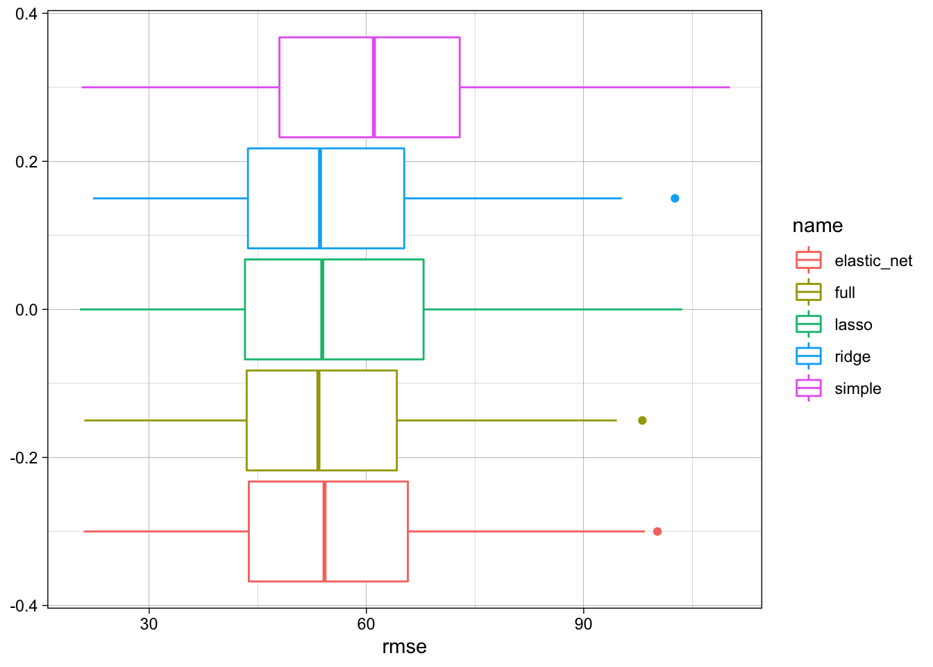
We see that the full model performs best, but the regularized models do not perform much worse.
simulations %>%
  dplyr::group_by(name) %>%
  dplyr::summarise(rmse_q90 = quantile(rmse, probs = 0.9),
                   rmse = median(rmse)) %>%
  dplyr::ungroup() %>%
  dplyr::mutate(perc = rmse / min(rmse)) %>%
  dplyr::arrange(perc)
## # A tibble: 5 × 4
##   name        rmse_q90  rmse  perc
##   <fct>          <dbl> <dbl> <dbl>
## 1 full            72.5  53.4  1
## 2 ridge           74.4  53.6  1.00
## 3 lasso           76.5  53.9  1.01
## 4 elastic_net     74.1  54.2  1.02
## 5 simple          83.9  61.0  1.14
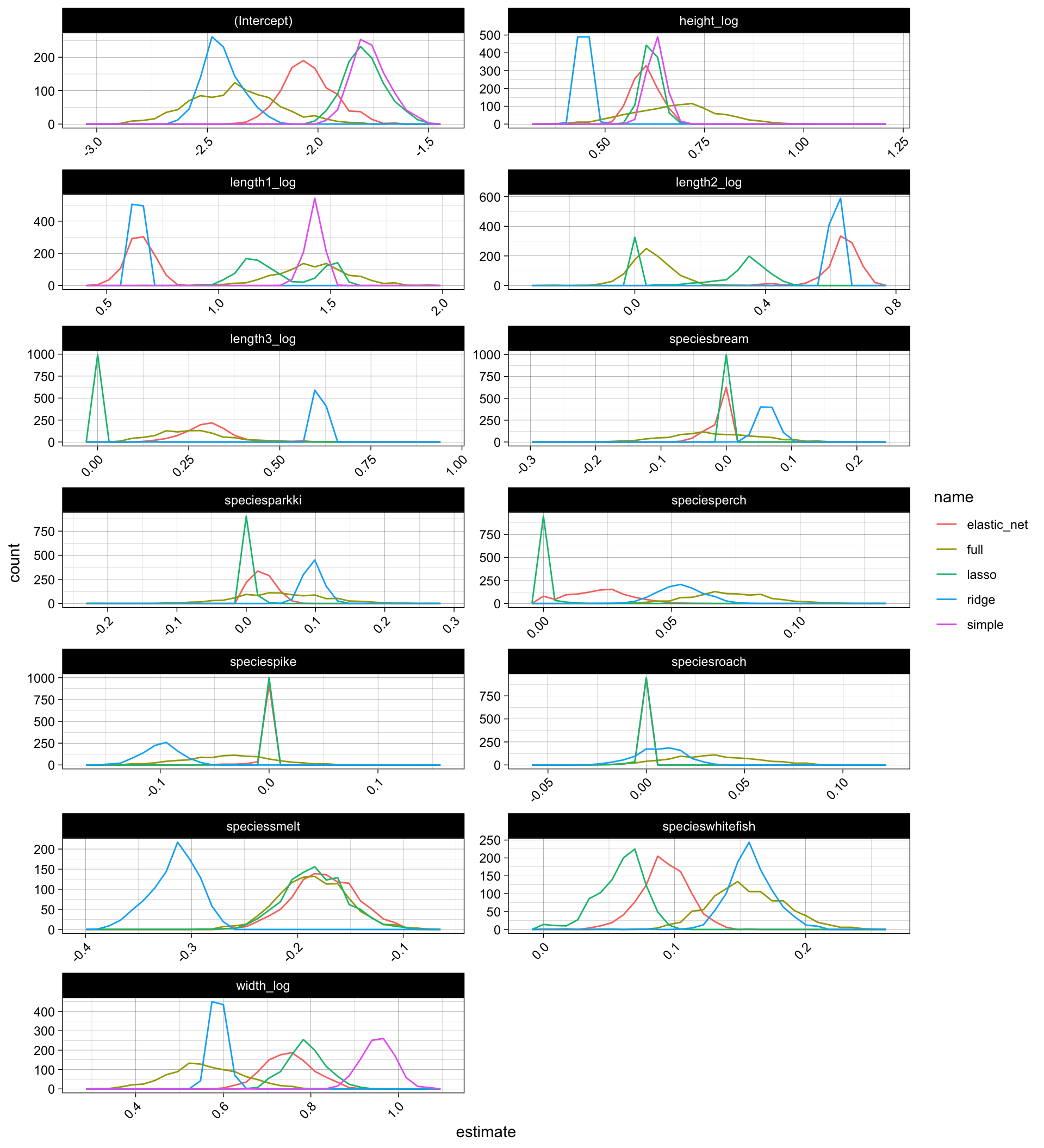
The coefficients though vary alot with respect to the different models but also the different simulations, especiall for the full model:
model_coefs <-
  simulations %>%
  dplyr::select(name, coefs) %>%
  tidyr::unnest(coefs)

model_coefs %>%
  ggplot(aes(x = estimate, color = name)) +
  geom_freqpoly(bins = 30) +
  facet_wrap(~ term, scales = "free", ncol = 2) +
  theme(axis.text.x = element_text(angle = 45, hjust = 1))
Conclusion 🔗
We saw how multicollinearity can cause trouble to the parameter estimation in linear regression, for example finding expression in high variance of parameters or lack of statistical significance. At the same time we saw that this does not necessarily lead to worse model performance in terms of test error metrics like root mean squared error.
We also learned about a couple of classical techniques to tackle these issues, for example looking at variance inflation factors, doing simple feature selection or applying regularization. There are many other helpful techniques, like dimensionality reduction, stepwise or tree-based feature selection.
Moreover many other more sophisticated machine learning models are more robust to these issues, as they incorporate information gain and regularization during the fit or use different data representations which are less vulnerable to single observations and correlation within the data. For example non-parametric candidates like tree models and sometimes also “extremely-parametric” models like neural networks.
But since linear regression allows us to draw strong insights and conclusions from data and is often useful as a naive benchmark model, it is very helpful to understand its statistical backbone and some of its drawbacks.