In the following post I want to give some impressions on how historic travel time data can be used to build a model for travel time estimations. In case you are are collecting your own characteristic travel data the you might actually be able to beat third-party-solutions in terms of accuracy as well as cost.
We will see why tree models might be suitable for this use case and we will do some feature engineering to improve the model performance.
Using tree based models 🔗
Let us look at some homemade toy data first, to see how a tree based model might be able to learn travel times. We assume a simple 2-dimensional space sized 10 times 10, where travelling from one coordinate to another can be done as the crow flies, so the distance in terms of time can be computed using the Pythagorean theorem (euclidean distance).
We store all possible combinations (x1, y1) to (x2, y2) and compute their distances:
## Built with python 3.6.15 with following packages:
## scikit-learn==0.23.2
## pandas==0.25.3
## seaborn==0.8.1
## numpy==1.19.0
## matplotlib==1.5.3
## pyproj==2.6.1
## lightgbm==2.3.1
## xgboost==0.90
import pandas as pd
from itertools import product
import numpy as np


prod = product(range(0, 10), range(0, 10))
xy = pd.DataFrame([p for p in prod], columns=['x', 'y'])

# cross join
xy_copy = xy.copy()
xy['_key'] = 1
xy_copy['_key'] = 1
data = pd.merge(xy, xy_copy, on='_key', suffixes = ('1', '2')).drop('_key', axis=1)

data.head(10)
##    x1  y1  x2  y2
## 0   0   0   0   0
## 1   0   0   0   1
## 2   0   0   0   2
## 3   0   0   0   3
## 4   0   0   0   4
## 5   0   0   0   5
## 6   0   0   0   6
## 7   0   0   0   7
## 8   0   0   0   8
## 9   0   0   0   9
def calculate_euclidean_distance(x1, y1, x2, y2):
    return np.sqrt(np.power(x2-x1, 2) + np.power(y2-y1, 2))

data['t'] = calculate_euclidean_distance(data['x1'], data['y1'], data['x2'], data['y2'])
To be able to visualize the travel time let us look at all trips from (0, 0) to all other locations. We first extract the relevant rows and then create a pivot table to be able to plot the data as a heatmap:
data_0_0 = data.loc[(data['x1'] == 0) & (data['y1'] == 0),:].copy()
import matplotlib
matplotlib.use('TkAgg')

import seaborn as sns
import matplotlib.pyplot as plt

data_0_0_piv = data_0_0.pivot('y2','x2','t')

ax = sns.heatmap(data_0_0_piv,
                 cmap='Blues',
                 robust=True)
ax = ax.invert_yaxis()
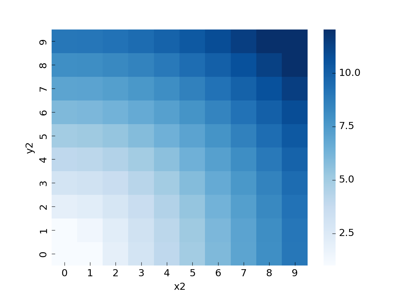
So if we want to travel from (0, 0) to (3, 3) it will cost around 4.2 (sqrt(3^2+3^2)), and so on. The pattern is essentially a quarter-circle around the origin.
Now as you know, decision trees are pretty much made to learn patterns as above, at least that is how they look at data: they partition the feature space (here: x and y, or more specifically x1, x2 and y1, y2) into rectangles (leafs).
Let us train a decision tree on the data and look how well it picks up the pattern. For a resilient test error we would need to split our dataset into train and test in a spatial manner, for the visualization we will skip this step though:
from sklearn.tree import DecisionTreeRegressor
dtr = DecisionTreeRegressor(max_depth=7, min_samples_leaf=5, random_state=30)

x, y = data[['x1', 'y1', 'x2', 'y2']], data['t']
_ = dtr.fit(x, y)

data_0_0['t_pred'] = dtr.predict(data_0_0[['x1', 'y1', 'x2', 'y2']])
data_0_0_pred = data_0_0.pivot('y2','x2','t_pred')

ax = sns.heatmap(data_0_0_pred,
                 cmap='Blues',
                 robust=True)
ax = ax.invert_yaxis()
plt.show()
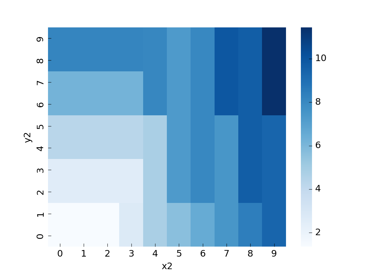
You can see that all areas have at least size 5 (min_samples_leaf).
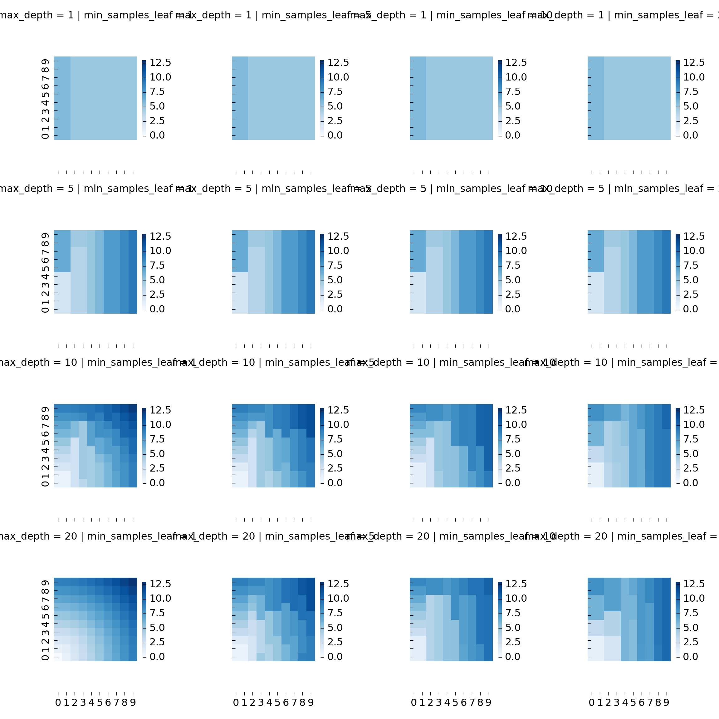
Let us generate a few more trees with different parameters to get a better picture:
import itertools

params = {
    'max_depth': [1,5,10,20],
    'min_samples_leaf': [1,5,10,20],
}

keys = params.keys()
values = (params[key] for key in keys)

params_list = [dict(zip(keys, p)) for p in itertools.product(*values)]
params_list now looks like this:
## [{'max_depth': 1, 'min_samples_leaf': 1}, {'max_depth': 1, 'min_samples_leaf': 5}, {'max_depth': 1, 'min_samples_leaf': 10}, {'max_depth': 1, 'min_samples_leaf': 20}, {'max_depth': 5, 'min_samples_leaf': 1}, {'max_depth': 5, 'min_samples_leaf': 5}, {'max_depth': 5, 'min_samples_leaf': 10}, {'max_depth': 5, 'min_samples_leaf': 20}, {'max_depth': 10, 'min_samples_leaf': 1}, {'max_depth': 10, 'min_samples_leaf': 5}, {'max_depth': 10, 'min_samples_leaf': 10}, {'max_depth': 10, 'min_samples_leaf': 20}, {'max_depth': 20, 'min_samples_leaf': 1}, {'max_depth': 20, 'min_samples_leaf': 5}, {'max_depth': 20, 'min_samples_leaf': 10}, {'max_depth': 20, 'min_samples_leaf': 20}]
data_list = []

for params in params_list:
    dtr = DecisionTreeRegressor(**params, random_state=1234)
    dtr = dtr.fit(x, y)

    data_0_0['t_pred'] = dtr.predict(data_0_0[['x1', 'y1', 'x2', 'y2']])

    data_0_0_p = data_0_0.pivot('y2','x2','t_pred')

    for key, value in params.items():
        data_0_0_p[key] = value

    data_list.append(data_0_0_p)

data = pd.concat(data_list)
We can plot all heatmaps using FacetGrid and a helper function:
def heatmap_view(**kwargs):
    kwargs['data'] = kwargs['data'].iloc[0:10,0:10]
    ax = sns.heatmap(
        **kwargs,
        cmap='Blues',
        vmin=0,
        vmax=13,
        square=True,
        cbar_kws={"shrink": .5}
    )
    return ax.invert_yaxis()

g = sns.FacetGrid(data, row='max_depth', col='min_samples_leaf')
g = g.map_dataframe(heatmap_view)
Geospatial features: haversine distance and azimuth 🔗
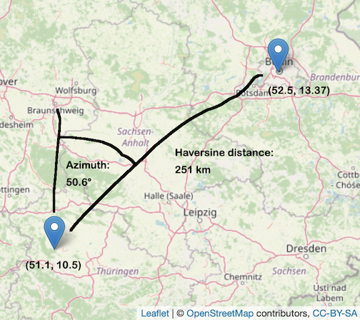
Two plausible geospatial features are haversine distance (shortest distance between 2 points on a sphere, here assuming Earth-radius) and azimuth (describes an angle between 2 coordinates).
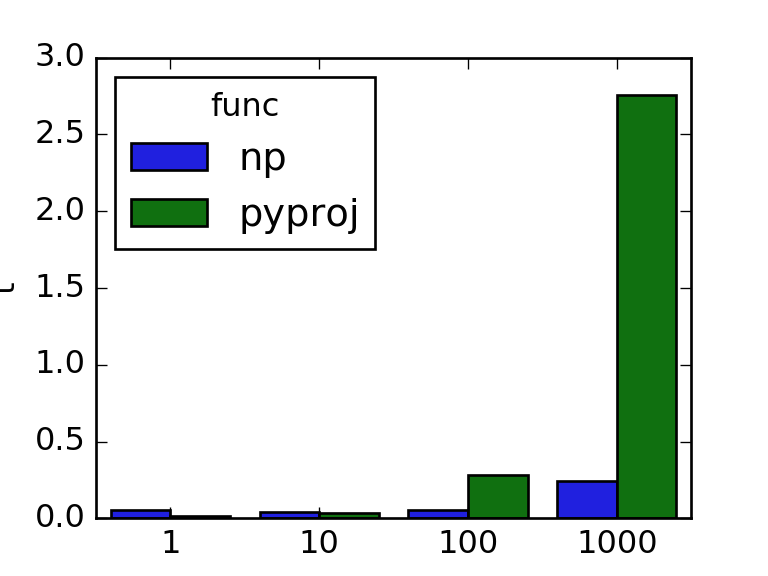
We can theoretically compute both metrics using pyproj, but we will see that plain numpy implementations perform better for calls on arrays.
Let us first compute (forward) azimuth, back azimuth and distance between Berlin and a national park in the middle of Germany using pyproj.Geod:
from pyproj import Geod

geodesic = Geod(ellps='clrk66')
azimuth, backward_azimuth, haversine_distance = geodesic.inv(10.5, 51.1, 13.37, 52.5)
azimuth, haversine_distance
## (50.68448458832755, 251888.26670165634)
The numpy equivalent functions can be defined as follows, the haversine for example as following way:
def calculate_haversine_distance(lat1, lon1, lat2, lon2):
    lon1, lat1, lon2, lat2 = map(np.radians, [lon1, lat1, lon2, lat2])

    dlon = lon2 - lon1
    dlat = lat2 - lat1

    a = np.sin(dlat/2.0)**2 + np.cos(lat1) * np.cos(lat2) * np.sin(dlon/2.0)**2

    c = 2 * np.arcsin(np.sqrt(a))
    m = 6367 * 1000 * c
    return m

calculate_haversine_distance(51.1, 10.5, 52.5, 13.37) # = 251.xxx
## 251169.9510116781
The following function can be used to compute the azimuth (also called compass bearing) according to this gist:
def calculate_azimuth(lat1, lon1, lat2, lon2):
    lat1_rad = np.radians(lat1)
    lat2_rad = np.radians(lat2)

    lon_delta = np.radians(lon2 - lon1)
    x = np.sin(lon_delta) * np.cos(lat2_rad)
    y = np.cos(lat1_rad) * np.sin(lat2_rad) - (np.sin(lat1_rad)
            * np.cos(lat2_rad) * np.cos(lon_delta))

    initial_bearing_rad = np.arctan2(x, y)
    initial_bearing = np.degrees(initial_bearing_rad)
    compass_bearing = (initial_bearing + 360) % 360
    return compass_bearing

calculate_azimuth(51.1, 10.5, 52.5, 13.37) # = 50.6x
## 50.61201583089286
Let us now compare the pyproj and numpy variants for arrays of length 1, 10, 100 and 1000, using timeit. For a fairer comparison we will place the constructor call to Geod in the global scope:
import timeit
from pyproj import Geod

geodesic = Geod(ellps='clrk66')

def calculate_azimuth_haversine_distance_np(lon1, lat1, lon2, lat2):
    return calculate_azimuth(lon1, lat1, lon2, lat2), calculate_haversine_distance(lon1, lat1, lon2, lat2)

def calculate_azimuth_haversine_distance_pyproj(lon1, lat1, lon2, lat2):
    azimuth, _, haversine_distance = geodesic.inv(lon1, lat1, lon2, lat2)
    return azimuth, haversine_distance

def time_func(func, n):
    lat1, lon1 = np.repeat(51.1, n), np.repeat(10.5, n)
    lat2, lon2 = np.repeat(52.5, n), np.repeat(13.37, n)
    number = 100
    # timeit evaluates in s, we return ms
    return timeit.timeit(
        stmt=f'calculate_azimuth_haversine_distance_{func}(lat1, lon1, lat2, lon2)',
        number=number,
        setup='from __main__ import calculate_azimuth_haversine_distance_np, calculate_azimuth_haversine_distance_pyproj',
        globals=locals()
    ) / number * 1000
import matplotlib.pyplot as plt
from itertools import product
import pandas as pd
import seaborn as sns

n = np.power(10, range(4))
prod = product(['np', 'pyproj'], n)
df = pd.DataFrame([p for p in prod], columns=['func', 'n'])

df['t'] = df.apply(lambda row: time_func(func=row['func'], n=row['n']), axis=1)

plt.figure(figsize=(4,3))
## <matplotlib.figure.Figure object at 0x128342908>
ax = sns.barplot(x='n', y='t', hue='func', data=df)
plt.show()
If we want to add these computed features to our coordinates now, we could for example create sklearn transformer. We will base our transformers on pandas, although in general, if you want to productionize your code it is good practice to use numpy arrays for performance reasons. In general those are a bit more challenging to work with, because you need to keep state of the column names if you want to extract things like feature importance.
from sklearn.base import BaseEstimator, TransformerMixin
from typing import Callable
import pandas as pd

class GeoTransformer(BaseEstimator, TransformerMixin):
    def __init__(self,
                 name,
                 func: Callable[[float, float, float, float], float],
                 lat1='pickup_latitude', lon1='pickup_longitude', lat2='dropoff_latitude', lon2='dropoff_longitude'):
        self.name = name
        self.func = func

        self.lat1 = lat1
        self.lon1 = lon1
        self.lat2 = lat2
        self.lon2 = lon2

    def fit(self, X: pd.DataFrame, y: pd.Series=None):
        # nothing to do here
        return self

    def transform(self, X: pd.DataFrame, y: pd.Series=None) -> pd.DataFrame:
        df = X.copy()
        df[self.name] = self.func(
            lat1=X[self.lat1],
            lon1=X[self.lon1],
            lat2=X[self.lat2],
            lon2=X[self.lon2],
        )
        return df
Again, let us also define some toy data to see test the transformers:
data = pd.DataFrame({
  'pickup_location': ['National park', 'Museum of Photography', 'Museum of Photography', ],
  'dropoff_location': ['Random location in Berlin', 'Alexanderplatz', 'Treptow Harbour'],
  'pickup_latitude': [51.1, 52.5033067, 52.5033067],
  'pickup_longitude': [10.5, 13.3403941, 13.3403941],
  'dropoff_latitude': [52.5, 52.5236452, 52.4937243],
  'dropoff_longitude': [13.37, 13.4042092, 13.4472089],
  'pickup_datetime': pd.to_datetime(['2020-06-18 12:30:00', '2020-06-21 13:45:00', '2020-06-21 14:00:00'])
})
##          pickup_location  ...     pickup_datetime
## 0          National park  ... 2020-06-18 12:30:00
## 1  Museum of Photography  ... 2020-06-21 13:45:00
## 2  Museum of Photography  ... 2020-06-21 14:00:00
##
## [3 rows x 7 columns]
hd_transformer = GeoTransformer(name='haversine_distance', func=calculate_haversine_distance)
hd_transformer.fit_transform(data)
##          pickup_location  ... haversine_distance
## 0          National park  ...      251169.951012
## 1  Museum of Photography  ...        4871.679462
## 2  Museum of Photography  ...        7304.160510
##
## [3 rows x 8 columns]
a_transformer = GeoTransformer(name='azimuth', func=calculate_azimuth)
a_transformer.fit_transform(data)
##          pickup_location  ...    azimuth
## 0          National park  ...  50.612016
## 1  Museum of Photography  ...  62.333692
## 2  Museum of Photography  ...  98.340432
##
## [3 rows x 8 columns]
In a similar fashion we could also add some datetime parts like hour, weekday, day and month, for example to capture traffic trends and seasonalities during the day or even the year.
from sklearn.base import BaseEstimator, TransformerMixin
import pandas as pd

class DatetimeTransformer(BaseEstimator, TransformerMixin):
    cols = ['hour', 'weekday', 'day', 'month']

    def __init__(self, col: str):
        self.col = col

    def fit(self, X: pd.DataFrame, y: pd.Series=None):
        # nothing to do here
        return self

    def transform(self, X: pd.DataFrame, y: pd.Series=None) -> pd.DataFrame:
        X.loc[:,'hour'] = X[self.col].dt.hour
        X.loc[:,'weekday'] = X[self.col].dt.weekday
        X.loc[:,'day'] = X[self.col].dt.day
        X.loc[:,'month'] = X[self.col].dt.month
        return X
dt_transformer = DatetimeTransformer(col='pickup_datetime')
dt_transformer.fit_transform(data)
##          pickup_location           dropoff_location  ...  day  month
## 0          National park  Random location in Berlin  ...   18      6
## 1  Museum of Photography             Alexanderplatz  ...   21      6
## 2  Museum of Photography            Treptow Harbour  ...   21      6
##
## [3 rows x 11 columns]
Lastly we will add a transformer to select specific columns to explore and compare the different features:
from typing import List
import pandas as pd

class ColumnSelector(BaseEstimator, TransformerMixin):
    def __init__(self, cols: List[str]):
        self.cols = cols

    def fit(self, X: pd.DataFrame, y: pd.Series=None):
        return self

    def transform(self, X: pd.DataFrame, y: pd.Series=None) -> pd.DataFrame:
        return X[self.cols]
Training a model 🔗
In a previous post we have worked with New York taxi data, containing pickup- and dropoff-coordinates as well as trip durations.
Let us extract a few random trips, we can use the following query, store the result as a csv file and load it using pandas:
WITH raw_data AS
(
  SELECT
    pickup_datetime,
    pickup_latitude,
    pickup_longitude,
    dropoff_latitude,
    dropoff_longitude,
    DATETIME_DIFF(dropoff_datetime, pickup_datetime, SECOND) AS duration
  FROM `bigquery-public-data.new_york_taxi_trips.tlc_yellow_trips_2016`
  WHERE
    pickup_latitude BETWEEN -90 AND 90
    AND pickup_longitude IS NOT NULL
    AND dropoff_latitude BETWEEN -90 AND 90
    AND dropoff_longitude IS NOT NULL
),
filtered_data AS
(
  SELECT
    *
  FROM raw_data
  WHERE
    duration BETWEEN 60 AND 60 * 60 * 6
    AND ST_DISTANCE(ST_GEOGPOINT(pickup_longitude, pickup_latitude), ST_GEOGPOINT(dropoff_longitude, dropoff_latitude)) BETWEEN 100 AND 25000
)
SELECT
  *
FROM filtered_data
WHERE
  RAND() < 200000 / (SELECT COUNT(*) FROM filtered_data)
data = pd.read_csv("../../../static/data/bigquery/bigquery_public_data_new_york_taxi_trips_tlc_yellow_trips_2016_sample.csv.gz",
                   parse_dates=['pickup_datetime']).sample(200000)
To evaluate the model we will create we should split the data. We will split the data randomly, which is somewhat naive in our use case, since the model can learn from almost identical coordinates which most likely exist in the data. If we want to evaluate how well the model performs on new areas we could split the data geographically, to estimate how well the model can abstract geographies and apply them to new areas. For that use case the model will perform rather poorly.
To make the model more robust for edge and outlier cases, or in general cases outside of the supported area, it can make sense to create a fallback model as proposed in one of my previous blog posts. In any case features like haversine distance and azimuth (direction) will help the model to to abstract estimates from or to unknown coordinates up to some degree.
Moreover we will define root mean squared error as our error metric, to penalize large errors more, but we will also look at mean absolute error for improved interpretability.
from sklearn.model_selection import train_test_split
from sklearn.metrics import mean_squared_error, mean_absolute_error
import numpy as np

def rmse(y_true, y_pred):
    return np.round(np.sqrt(mean_squared_error(y_true=y_true, y_pred=y_pred)), 2)

def mae(y_true, y_pred):
    return np.round(mean_absolute_error(y_true=y_true, y_pred=y_pred), 2)

col_target = 'duration'
cols_features = ['pickup_latitude', 'pickup_longitude',
                 'dropoff_latitude', 'dropoff_longitude',
                 'pickup_datetime']

x_train, x_test, y_train, y_test = train_test_split(data[cols_features], data[col_target])
Let us now try to get an estimate of how good a linear model performs on the data, also to compare it to the nonlinear models later. Instead of simply using the pickup and dropoff coordinates as features we can k-bins-discretize them to allow the model to learn some kind of grid pattern:
from sklearn.pipeline import Pipeline
from sklearn.preprocessing import KBinsDiscretizer
from sklearn.compose import ColumnTransformer
from sklearn.linear_model import Ridge

cols_features = ['pickup_latitude', 'pickup_longitude', 'dropoff_latitude', 'dropoff_longitude',
                 'hour', 'weekday', 'day', 'month',
                 'haversine_distance', 'azimuth']
cols_coordinates = ['pickup_longitude', 'pickup_latitude', 'dropoff_longitude', 'dropoff_latitude']

k_bins_discretizer = ColumnTransformer([
    ('k_bins_discretizer', KBinsDiscretizer(n_bins=16, encode='onehot-dense'), cols_coordinates),
], remainder='drop')

pipeline = Pipeline([
    ('haversine_distance', GeoTransformer(name='haversine_distance', func=calculate_haversine_distance)),
    ('azimuth', GeoTransformer(name='azimuth', func=calculate_haversine_distance)),
    ('datetime', DatetimeTransformer(col='pickup_datetime')),
    ('column_selector', ColumnSelector(cols=cols_features)),
    ('k_bins_discretizer', k_bins_discretizer),
    ('model', Ridge())
])

_ = pipeline.fit(x_train, y_train)
y_pred = pipeline.predict(x_test)
rmse(y_pred=y_pred, y_true=y_test), mae(y_pred=y_pred, y_true=y_test)
## (559.06, 398.98)
We can see that applying the KBinsDiscretizer actually makes the predictions worse:
from sklearn.model_selection import GridSearchCV

cv = GridSearchCV(pipeline, param_grid = {'k_bins_discretizer': ['passthrough', k_bins_discretizer]})
_ = cv.fit(x_train, y_train)
y_pred = cv.predict(x_test)

rmse(y_pred=y_pred, y_true=y_test), mae(y_pred=y_pred, y_true=y_test)
## (401.83, 276.81)
cv.best_params_
## {'k_bins_discretizer': 'passthrough'}
Let us now create a generic pipeline to compare different models, like xgboost, LightGBM and also two native sklearn implementations.
from sklearn.pipeline import Pipeline

def create_pipeline(model):
    cols_features = ['pickup_latitude', 'pickup_longitude', 'dropoff_latitude', 'dropoff_longitude',
                     'hour', 'weekday', 'day', 'month',
                     'haversine_distance', 'azimuth']

    pipeline = Pipeline([
        ('haversine_distance', GeoTransformer(name='haversine_distance', func=calculate_haversine_distance)),
        ('azimuth', GeoTransformer(name='azimuth', func=calculate_haversine_distance)),
        ('datetime', DatetimeTransformer(col='pickup_datetime')),
        ('column_selector', ColumnSelector(cols=cols_features)),
        ('model', model)
    ])

    return pipeline
LightGBM has the advantage that it can handle categorical features quite well, without the necessity of one-hot-encoding. In general one-hot-encoding should be applied carefully in tree models, especially for variables with higher cardinality - you can find a good explanation in this blog post. In our case we will not apply one-hot-encoding to the categorical variables like weekday or hour. Alternatively cyclical encoding could be applied, to avoid sparsity and independence of the dummified features introduced by naive one-hot-encoding.
from lightgbm.sklearn import LGBMRegressor
from sklearn.linear_model import Ridge
from sklearn.ensemble import GradientBoostingRegressor, RandomForestRegressor
from xgboost import XGBRegressor

models = {
    'LGBMRegressor': LGBMRegressor(importance_type='gain'),
    'GradientBoostingRegressor': GradientBoostingRegressor(),
    'RandomForestRegressor': RandomForestRegressor(),
    'XGBRegressor': XGBRegressor(objective='reg:squarederror'),
    'Ridge': Ridge(),
}
Let us now create pipelines for each model and evaluate them using our test data:
import time

pipelines = {}

for model_name, model in models.items():
    pipeline = create_pipeline(model)

    t = time.time()
    _ = pipeline.fit(x_train, y_train)
    pipelines[model_name] = pipeline

    y_pred = pipeline.predict(x_test)

    metrics = {
      'rmse': rmse(y_pred=y_pred, y_true=y_test),
      'mae': mae(y_pred=y_pred, y_true=y_test),
      'fit_time': np.round(time.time() - t, 2)
    }

    print(f'{model_name}: {metrics}')
## LGBMRegressor: {'rmse': 299.21, 'mae': 196.23, 'fit_time': 1.18}
## GradientBoostingRegressor: {'rmse': 332.25, 'mae': 219.75, 'fit_time': 34.99}
## RandomForestRegressor: {'rmse': 303.28, 'mae': 197.26, 'fit_time': 140.97}
## XGBRegressor: {'rmse': 332.9, 'mae': 220.31, 'fit_time': 12.15}
## Ridge: {'rmse': 401.83, 'mae': 276.81, 'fit_time': 0.3}
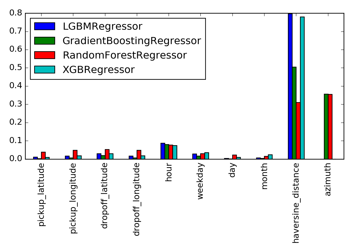
Let us extract (and normalize) and compare the feature importances:
feature_importances = {
    model_name: pipeline.named_steps['model'].feature_importances_ / sum(pipeline.named_steps['model'].feature_importances_)
    for model_name, pipeline in pipelines.items()
    if hasattr(pipeline.named_steps['model'], 'feature_importances_')
}

feature_importances_df = pd.DataFrame(feature_importances, index=cols_features)
feature_importances_df.plot(kind='bar')
## <matplotlib.axes._subplots.AxesSubplot object at 0x127f229e8>
We can quickly take a look at the performance of the full pipelines, to get a rough estimate:
import timeit

n = 100
rows = 10

for model_name, pipeline in pipelines.items():
    t = timeit.timeit(stmt='pipeline.predict(x_test.iloc[0:rows,:])',
                      globals=globals(),
                      number=n) / n
    print(f'{model_name}: {t * 1000:.1f}ms')
## LGBMRegressor: 56.1ms
## GradientBoostingRegressor: 31.8ms
## RandomForestRegressor: 61.4ms
## XGBRegressor: 28.9ms
## Ridge: 30.4ms
Now let us take a look at some predictions by visualizing them using Uber’s kepler.gl. We can for example pick a random pickup location and make predictions for many different dropoff locations and map these onto a choropleth map.
We can use pyproj again to map some corner coordinates into a flat space (and back), generate a grid with points of equal distance and then convert the points back.
from pyproj import Transformer
import numpy as np

# define a grid using lat longs of south-west and north-east corners and step size in meters
def create_grid(sw_lon, sw_lat, ne_lon, ne_lat, step_size):
    transformer = Transformer.from_crs("epsg:4326", "epsg:3857", always_xy=True)
    sw_lon_transformed, sw_lat_transformed = transformer.transform(sw_lon, sw_lat)
    ne_lon_transformed, ne_lat_transformed = transformer.transform(ne_lon, ne_lat)

    # create actual grid
    x = np.arange(sw_lon_transformed, ne_lon_transformed, step_size)
    y = np.arange(sw_lat_transformed, ne_lat_transformed, step_size)
    xx, yy = np.meshgrid(x, y)

    lons, lats = transformer.transform(xx.ravel(), yy.ravel(), errcheck=True, direction='inverse')
    return lons, lats
lons, lats = create_grid(sw_lon=-74.031216,  sw_lat=40.741904,  ne_lon=-73.893833, ne_lat=40.807015,  step_size=200)

grid = pd.DataFrame({
    'pickup_datetime': pd.to_datetime('2020-06-20 12:30:00'),
    'pickup_latitude': 40.770880,
    'pickup_longitude': -73.949176,
    'dropoff_latitude': lats,
    'dropoff_longitude': lons,
})
We can now get our pipeline using the LightGBM regressor and do some predictions:
pipeline = pipelines['LGBMRegressor']
grid['y_pred'] = pipeline.predict(grid)
grid.sample(10)
##          pickup_datetime  pickup_latitude  ...  dropoff_longitude       y_pred
## 3118 2020-06-20 12:30:00         40.77088  ...         -73.962944   701.220479
## 437  2020-06-20 12:30:00         40.77088  ...         -73.937791   755.670820
## 685  2020-06-20 12:30:00         40.77088  ...         -73.907248  1071.559425
## 2315 2020-06-20 12:30:00         40.77088  ...         -74.022233  1881.329286
## 2247 2020-06-20 12:30:00         40.77088  ...         -74.006063  1433.173588
## 488  2020-06-20 12:30:00         40.77088  ...         -73.984504  1193.817610
## 3173 2020-06-20 12:30:00         40.77088  ...         -74.002470  1384.050994
## 526  2020-06-20 12:30:00         40.77088  ...         -73.916232  1017.198240
## 301  2020-06-20 12:30:00         40.77088  ...         -73.905452  1123.225951
## 3564 2020-06-20 12:30:00         40.77088  ...         -73.991690  1354.784517
##
## [10 rows x 6 columns]
Finally we can export the grid precitions to a file and upload it to kepler.gl. I’ve prepared a animated visualization of the grid, where the grid cells are colored depending on the predicted value (red to yellow, low to high):

We can see that the model learns a circular pattern, and also some street topology. But can we also incorporate bridges, highways, etc? For example by either using the taxi zones provided as another public dataset, or alternatively by applying clustering first and use the assigned cluster as a feature. Since our data originates from New York we could also use manhatten metric, as the streets are well structured and follow a grid layout. Some of these challenges will be tackled in a second part.
Update from 2020-06-25: In case you are interested, a few days ago an excellent blog post on the same topic was published via medium. Using Gaussian mixtures as clustering is a very good approach, as the cluster assignment can be done very fast.