We will work on a public dataset (actually two) of yellow taxi trips in New York. The dataset contains individual taxi trips with start- and endtimes, pickup- and dropoff-locations, number of passengers and some other data. Two datasets, because we will union the to datasets of trips in 2017 and 2018 into one table to make the problem a bit more interesting in terms of scale!
To reduce cost and make querying more efficient we partition the table by the date of pickup, and cluster it by vendor and locations. Additionally we add an id to make debugging easier.
CREATE OR REPLACE TABLE temp.nyc_taxi_trips_raw
PARTITION BY pickup_date
CLUSTER BY vendor_id, pickup_location_id, dropoff_location_id
AS
SELECT
  * EXCEPT (pickup_longitude, pickup_latitude, dropoff_longitude, dropoff_latitude),
  DATE(pickup_datetime) AS pickup_date,
  GENERATE_UUID() AS _id
FROM `bigquery-public-data.new_york_taxi_trips.tlc_yellow_trips_2017`
UNION ALL
SELECT
  *,
  DATE(pickup_datetime) AS pickup_date,
  GENERATE_UUID() AS _id
FROM `bigquery-public-data.new_york_taxi_trips.tlc_yellow_trips_2018`
Query complete (1 min 16 sec elapsed, 36.5 GB processed)
The storage of this table costs around 0.80$ per month (20$ per 1 TB per month). Any table or partition not touched for 90 days goes into long term storage, without any degrading of service, but the cost of storage actually halves. Creating the table itself (scanning the data) costs around 0.20$ (5$ per 1 TB). Almost all queries that we run below will scan around similar or much lower amounts of data, although we will run queries on around 200 million rows. Since BigQuery stores data columnnar (see Google’s An Inside Look at Google BigQuery), we can reduce the amount of data scanned by only selecting and using the columns we need.
To run queries on the data we either
- create a connection via
DBI::dbConnectand then register our table usingdplyr::tblon the connection and the table name, to query it usingdplyrverbs, or - we can write plain SQL and fetch the result set using
DBI::dbGetQueryas in theget_bq_datafunction below.
#' create connection to bq project
#' @param project_id id of the project
#' @return a connection object
create_bq_connection <- function(project_id = Sys.getenv("GCP_PROJECT_ID")) {
  con <- DBI::dbConnect(drv = bigrquery::bigquery(),
                        project = project_id,
                        billing = project_id,
                        quiet = FALSE)
}

#' fetch data from bq
#' @param query a query string
#' @param project_id id of the project
#' @return return data as dplyr::tibble
get_bq_data <- function(query, project_id = Sys.getenv("GCP_PROJECT_ID")) {
  con <- create_bq_connection(project_id)

  start_time <- Sys.time()
  data <- DBI::dbGetQuery(con, query)
  time_elapsed <- round(difftime(Sys.time(), start_time, units = "secs"), 2)
  message("Fetched: ", nrow(data), " rows")
  message("Elapsed: ", time_elapsed, " s")
  return(dplyr::as_tibble(data))
}
query <- "
  SELECT
    COUNT(*) AS trips_sum,
    AVG(DATETIME_DIFF(dropoff_datetime, pickup_datetime, MINUTE)) AS trip_duration_avg,
    MAX(DATETIME_DIFF(dropoff_datetime, pickup_datetime, MINUTE)) AS trip_duration_max,
    AVG(trip_distance) AS trip_distance_avg,
    MAX(trip_distance) AS trip_distance_max,
    AVG(passenger_count) AS passenger_count_avg,
    MAX(passenger_count) AS passenger_count_max,
    MIN(pickup_datetime) AS pickup_datetime_min,
    MAX(pickup_datetime) AS pickup_datetime_max
  FROM temp.nyc_taxi_trips_raw
"
stats <- get_bq_data(query)
## Auto-refreshing stale OAuth token.
## Complete
## Billed: 0 B
## Fetched: 1 rows
## Elapsed: 3.88 s
## $trips_sum
## [1] 225731500
##
## $trip_duration_avg
## [1] 16.58556
##
## $trip_duration_max
## [1] 757771
##
## $trip_distance_avg
## [1] 2.92944
##
## $trip_distance_max
## [1] 189483.8
##
## $passenger_count_avg
## [1] 1.610483
##
## $passenger_count_max
## [1] 192
##
## $pickup_datetime_min
## [1] "2001-01-01 00:01:48 UTC"
##
## $pickup_datetime_max
## [1] "2084-11-04 12:32:24 UTC"
Our data contains a bit more than 200 million trips, and outliers in almost all important dimensions. Let us quickly aggregate the trips to dailies and plot them to get a feeling for the data:
query <- "
  SELECT
    pickup_date AS date,
    COUNT(*) AS trips
  FROM `temp.nyc_taxi_trips_raw`
  GROUP BY 1
"

data <- get_bq_data(query)
## Complete
## Billed: 0 B
## Fetched: 809 rows
## Elapsed: 3.13 s
summary(data)
##       date                trips
##  Min.   :2001-01-01   Min.   :     1
##  1st Qu.:2017-07-12   1st Qu.:260126
##  Median :2018-01-30   Median :297073
##  Mean   :2018-04-12   Mean   :279025
##  3rd Qu.:2018-08-20   3rd Qu.:325631
##  Max.   :2084-11-04   Max.   :699680
data %>%
  dplyr::filter(date >= "2017-01-01" & date <= "2018-12-31") %>%
  ggplot(aes(x = date, y = trips)) +
  geom_line()
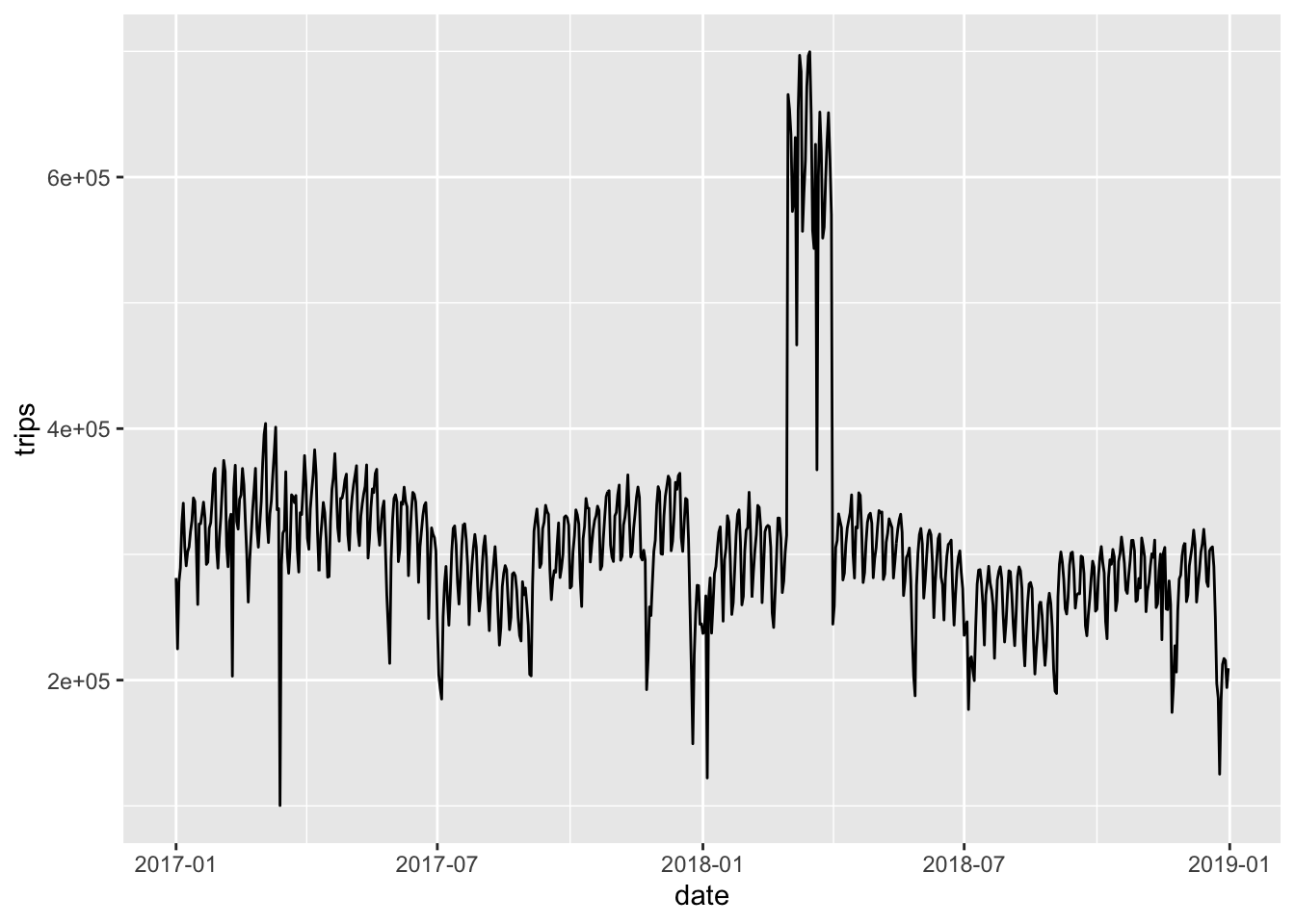
It seems like the input data contains some duplicates for certain periods, which we can verify by looking at individual trips. We can deduplicate it using trip start- and endtimes, distance and vendor and BigQuery’s ROW_NUMBER window function, where we add row numbers per partition. We will also remove trips with weird durations and out of the date ranges. In BigQuery we could theoretically even do this in place (as in CREATE OR REPLACE TABLE tbl AS SELECT * FROM tbl WHERE ...), but in our case we will create a new table.
CREATE OR REPLACE TABLE temp.nyc_taxi_trips
PARTITION BY pickup_date
CLUSTER BY vendor_id, pickup_location_id, dropoff_location_id AS
WITH trips_raw
AS
(
  SELECT
    *,
    ROW_NUMBER() OVER (PARTITION BY pickup_datetime, dropoff_datetime, vendor_id, trip_distance) AS _row_number
  FROM `temp.nyc_taxi_trips_raw`
  WHERE
    DATETIME_DIFF(dropoff_datetime, pickup_datetime, SECOND) BETWEEN 1 AND 1440
    AND DATE(pickup_datetime) BETWEEN '2017-01-01' AND '2018-12-31'
)
SELECT
  * EXCEPT (_row_number)
FROM trips_raw
WHERE
  _row_number = 1
Query complete (27.0 sec elapsed, 33.1 GB processed)
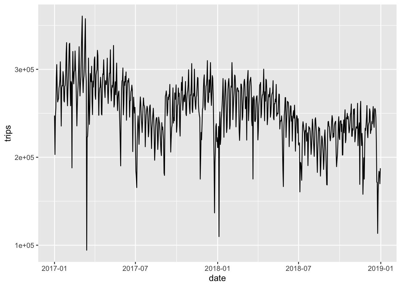
query <- "
  SELECT
    pickup_date AS date,
    COUNT(*) AS trips
  FROM `temp.nyc_taxi_trips`
  GROUP BY 1
"

data <- get_bq_data(query)
## Complete
## Billed: 0 B
## Fetched: 730 rows
## Elapsed: 3 s

data %>%
  dplyr::filter(date >= "2017-01-01" & date <= "2018-12-31") %>%
  ggplot(aes(x = date, y = trips)) +
  geom_line()
Whenever we want to investigate samples of data we should use the BigQuery preview - it is free! But we can also heavily reduce the amount of scanned data (and therefore cost) by selecting from a specific partition. The LIMIT itself does not reduce the amount of scanned data:
query <- "
  SELECT
    *
  FROM temp.nyc_taxi_trips
  WHERE
    pickup_date = '2018-07-01'
  ORDER BY 1,2,3
  LIMIT 5
"

data <- get_bq_data(query)
## Complete
## Billed: 0 B
## Fetched: 5 rows
## Elapsed: 2.64 s
## # A tibble: 5 × 19
##   vendor_id pickup_datetime     dropoff_datetime    passenger_count
##   <chr>     <dttm>              <dttm>                        <int>
## 1 1         2018-07-01 00:00:01 2018-07-01 00:03:47               1
## 2 1         2018-07-01 00:00:01 2018-07-01 00:04:59               1
## 3 1         2018-07-01 00:00:01 2018-07-01 00:07:07               2
## 4 1         2018-07-01 00:00:03 2018-07-01 00:03:16               3
## 5 1         2018-07-01 00:00:03 2018-07-01 00:15:16               1
## # … with 15 more variables: trip_distance <dbl>, rate_code <chr>,
## #   store_and_fwd_flag <chr>, payment_type <chr>, fare_amount <dbl>,
## #   extra <dbl>, mta_tax <dbl>, tip_amount <dbl>, tolls_amount <dbl>,
## #   imp_surcharge <dbl>, total_amount <dbl>, pickup_location_id <chr>,
## #   dropoff_location_id <chr>, pickup_date <date>, `_id` <chr>
## Rows: 5
## Columns: 19
## $ vendor_id           <chr> "1", "1", "1", "1", "1"
## $ pickup_datetime     <dttm> 2018-07-01 00:00:01, 2018-07-01 00:00:01, 2018-07-…
## $ dropoff_datetime    <dttm> 2018-07-01 00:03:47, 2018-07-01 00:04:59, 2018-07…
## $ passenger_count     <int> 1, 1, 2, 3, 1
## $ trip_distance       <dbl> 0.7, 1.2, 1.1, 0.6, 3.7
## $ rate_code           <chr> "1", "1", "1", "1", "1"
## $ store_and_fwd_flag  <chr> "N", "N", "N", "N", "N"
## $ payment_type        <chr> "1", "2", "1", "1", "2"
## $ fare_amount         <dbl> 5.0, 6.0, 6.5, 4.5, 14.5
## $ extra               <dbl> 0.5, 0.5, 0.5, 0.5, 0.5
## $ mta_tax             <dbl> 0.5, 0.5, 0.5, 0.5, 0.5
## $ tip_amount          <dbl> 1.40, 0.00, 1.55, 1.45, 0.00
## $ tolls_amount        <dbl> 0, 0, 0, 0, 0
## $ imp_surcharge       <dbl> 0.3, 0.3, 0.3, 0.3, 0.3
## $ total_amount        <dbl> 7.70, 7.30, 9.35, 7.25, 15.80
## $ pickup_location_id  <chr> "113", "140", "144", "236", "163"
## $ dropoff_location_id <chr> "107", "162", "249", "236", "179"
## $ pickup_date         <date> 2018-07-01, 2018-07-01, 2018-07-01, 2018-07-01, 2…
## $ `_id`               <chr> "06940a65-9168-4d1c-93ae-e13138ccf8e5", "8d323b98-…
Let us unleash BigQuery’s computational power and compute the number of trips in-flight per pickup location and minute. We can achieve this by unnesting individual trips into minute-level and then aggregate those per location and minute:
CREATE OR REPLACE TABLE temp.nyc_taxi_trips_grid
PARTITION BY DATE(datetime)
CLUSTER BY pickup_location_id
AS
SELECT
  pickup_location_id,
  datetime,
  COUNT(*) AS trips,
  SUM(passenger_count) AS passengers,
  ARRAY_AGG(_id) AS _ids
FROM temp.nyc_taxi_trips t,
UNNEST(
  GENERATE_TIMESTAMP_ARRAY(
    TIMESTAMP(DATETIME_TRUNC(pickup_datetime, MINUTE)),
    TIMESTAMP(DATETIME_TRUNC(dropoff_datetime, MINUTE)),
    INTERVAL 1 MINUTE
  )
) AS datetime
GROUP BY 1,2
Query complete (57.5 sec elapsed, 11.4 GB processed)
This takes a bit longer, but it scales well if the trips are kinda equally distributed over the partitions (dates here).
query <- "
  SELECT
    *
  FROM temp.nyc_taxi_trips_grid
  WHERE
    DATE(datetime) = '2018-07-02'
  LIMIT 100
"

data <- get_bq_data(query)
## Complete
## Billed: 0 B
## Fetched: 100 rows
## Elapsed: 2.93 s
## # A tibble: 100 × 5
##    pickup_location_id datetime            trips passengers `_ids`
##    <chr>              <dttm>              <int>      <int> <list>
##  1 116                2018-07-02 20:09:00     1          5 <chr [1]>
##  2 116                2018-07-02 20:10:00     1          5 <chr [1]>
##  3 116                2018-07-02 20:07:00     1          5 <chr [1]>
##  4 116                2018-07-02 20:08:00     1          5 <chr [1]>
##  5 116                2018-07-02 20:11:00     1          5 <chr [1]>
##  6 116                2018-07-02 20:12:00     1          5 <chr [1]>
##  7 1                  2018-07-02 11:39:00     1          3 <chr [1]>
##  8 1                  2018-07-02 11:40:00     1          3 <chr [1]>
##  9 13                 2018-07-02 01:00:00     1          1 <chr [1]>
## 10 13                 2018-07-02 01:01:00     1          1 <chr [1]>
## # … with 90 more rows
We could also query for specific ids using a WHERE-clause like 'be1f18ea-3565-4d2c-86fb-b8bce2a63213' IN UNNEST(_ids).
Let us try to solve a typical SQL island problem using BigQuery’s computational power. Let us try to find all connected intervals where more than 50 taxis are in flight, starting from a specific pickup location. We can use a very naive approach to find islands of times where certain conditions are satisfied when we query our minute-level table.
This can be achieved by selecting all minutes where more than 50 trips where in flight, adding the time differences to the previous and next minute with at least 50 trips to the rows. We can then select all those minutes where minutes_to_previous > 1 or null, since these are the beginnings of a closed interval. To these we join all minutes equal or later that have a gap of more than 1 minute to next, i.e. minutes_to_next > 1 - of all those the first one is the end of the interval.
This approach is very naive and would not work on many undistributed relational databases. The confidence in the power of BigQuery to work efficiently on minutely grained data allows us to avoid any complicated logic that filters and resolves overlaps of various kinds using CASE WHEN statements and complicated joins:
CREATE OR REPLACE TABLE temp.nyc_taxi_trips_interval
PARTITION BY DATE(start_datetime)
CLUSTER BY pickup_location_id
AS
WITH leads_lags AS
(
  SELECT
    *,
    TIMESTAMP_DIFF(datetime, LAG(datetime) OVER (PARTITION BY pickup_location_id ORDER BY datetime), MINUTE) AS minutes_to_previous,
    TIMESTAMP_DIFF(LEAD(datetime) OVER (PARTITION BY pickup_location_id ORDER BY datetime), datetime, MINUTE) AS minutes_to_next
  FROM temp.nyc_taxi_trips_grid
  WHERE
    trips >= 50
),
events AS
(
  SELECT
    t1.pickup_location_id,
    t1.datetime AS start_datetime,
    MIN(t2.datetime) AS end_datetime
  FROM leads_lags t1
  LEFT JOIN leads_lags t2
    ON t2.pickup_location_id = t1.pickup_location_id
    AND t2.datetime >= t1.datetime
    AND (t2.minutes_to_next > 1 OR t2.minutes_to_next IS NULL)
  WHERE
    t1.minutes_to_previous > 1 OR t1.minutes_to_previous IS NULL
  GROUP BY 1,2
)
SELECT
  pickup_location_id,
  start_datetime,
  end_datetime,
  TIMESTAMP_DIFF(end_datetime, start_datetime, MINUTE) AS duration
FROM events
Query complete (1 min 15 sec elapsed, 1.7 GB processed)
query <- "
  SELECT
    *
  FROM temp.nyc_taxi_trips_interval t
  WHERE
    duration >= 60
  ORDER BY 1,2
  LIMIT 10
"

data <- get_bq_data(query)
## Complete
## Billed: 0 B
## Fetched: 10 rows
## Elapsed: 2.89 s
## # A tibble: 10 × 4
##    pickup_location_id start_datetime      end_datetime        duration
##    <chr>              <dttm>              <dttm>                 <int>
##  1 100                2017-01-02 15:38:00 2017-01-02 16:40:00       62
##  2 100                2017-01-02 17:00:00 2017-01-02 19:29:00      149
##  3 100                2017-01-03 08:19:00 2017-01-03 09:59:00      100
##  4 100                2017-01-03 11:53:00 2017-01-03 13:23:00       90
##  5 100                2017-01-03 13:52:00 2017-01-03 16:24:00      152
##  6 100                2017-01-03 17:31:00 2017-01-03 19:48:00      137
##  7 100                2017-01-04 07:46:00 2017-01-04 09:46:00      120
##  8 100                2017-01-04 17:52:00 2017-01-04 19:55:00      123
##  9 100                2017-01-05 08:00:00 2017-01-05 10:07:00      127
## 10 100                2017-01-05 10:11:00 2017-01-05 11:15:00       64
To aggregate the data to a timeseries, for example on a 30-minute level, we first create a grid table, which will hold all locations and all 30-minute time bins of 2017 and 2018. Using the grid on the left hand side of the join we can make sure to produce a dense timeseries (so no timebin will be missing, even if there were no trips during that time bin):
CREATE OR REPLACE TABLE temp.nyc_taxi_timeseries
PARTITION BY date
CLUSTER BY location_id
AS
WITH timeseries AS
(
  SELECT
    datetime
  FROM
  UNNEST(
    GENERATE_TIMESTAMP_ARRAY(
      TIMESTAMP('2017-01-01 00:00:00'),
      TIMESTAMP('2018-12-31 23:30:00'),
      INTERVAL 30 MINUTE
    )
  ) AS datetime
)
SELECT
  z.zone_id AS location_id,
  DATE(ts.datetime) AS date,
  DATETIME(ts.datetime) AS datetime
FROM `bigquery-public-data.new_york_taxi_trips.taxi_zone_geom` z
CROSS JOIN timeseries ts
Query complete (13.1 sec elapsed, 1.2 KB processed)
We can now floor timestamps of pickups and dropoffs to 30 minutes and add them to the timeseries:
CREATE TEMPORARY FUNCTION floor_datetime(x DATETIME) AS
(
  DATETIME_ADD(
    DATETIME_TRUNC(x, HOUR),
    INTERVAL CAST(FLOOR(EXTRACT(MINUTE FROM x) / 30) * 30 AS INT64) MINUTE
  )
);

CREATE OR REPLACE TABLE temp.nyc_taxi_trips_timeseries
AS
WITH pickups AS
(
  SELECT
    pickup_location_id AS location_id,
    floor_datetime(pickup_datetime) AS datetime,
    COUNT(*) AS n
  FROM `temp.nyc_taxi_trips`
  GROUP BY 1,2
),
dropoffs AS
(
  SELECT
    dropoff_location_id AS location_id,
    floor_datetime(dropoff_datetime) AS datetime,
    COUNT(*) AS n
  FROM `temp.nyc_taxi_trips`
  GROUP BY 1,2
)
SELECT
  t.location_id,
  t.datetime,
  COALESCE(p.n, 0) AS pickups,
  COALESCE(d.n, 0) AS dropoffs
FROM temp.nyc_taxi_timeseries t
LEFT JOIN pickups p USING (location_id, datetime)
LEFT JOIN dropoffs d USING (location_id, datetime)
Query complete (32.5 sec elapsed, 4.5 GB processed)
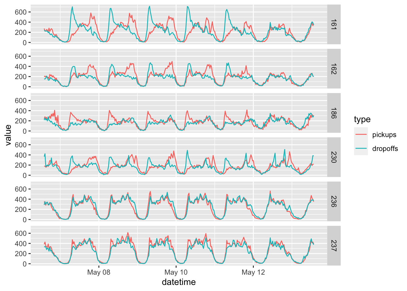
We will fetch a few sample timeseries and plot a week of half-hourly data, one location per panel:
query <- "
  SELECT
    location_id,
    datetime,
    pickups,
    dropoffs
  FROM temp.nyc_taxi_trips_timeseries
  WHERE
    location_id IN ('237', '161', '236', '162', '186', '230')
  ORDER BY 1,2,3
"

data <- get_bq_data(query)
## Complete
## Billed: 0 B
## Fetched: 210240 rows
## Elapsed: 4.57 s
data %>%
  dplyr::filter(datetime >= "2018-05-07" & datetime < "2018-05-14") %>%
  # convert wide to long
  tidyr::gather(type, value, -location_id, -datetime, factor_key = TRUE) %>%
  ggplot(aes(x = datetime, y = value, color = type)) +
  geom_line() +
  facet_grid(location_id ~ .)
In a similar way we can also compute and plot the timeseries per passenger counts:
query <- "
  CREATE TEMPORARY FUNCTION floor_datetime(x DATETIME) AS
  (
    DATETIME_ADD(
      DATETIME_TRUNC(x, HOUR),
      INTERVAL CAST(FLOOR(EXTRACT(MINUTE FROM x) / 30) * 30 AS INT64) MINUTE
    )
  );

  WITH pickups AS
  (
    SELECT
      pickup_location_id AS location_id,
      floor_datetime(pickup_datetime) AS datetime,
      CASE
        WHEN passenger_count <= 3 THEN CAST(passenger_count AS STRING)
        ELSE '4+'
      END AS passenger_count,
      COUNT(*) AS n
    FROM `temp.nyc_taxi_trips`
    GROUP BY 1,2,3
  )
  SELECT
    t.location_id,
    t.datetime,
    p.passenger_count,
    p.n AS pickups
  FROM temp.nyc_taxi_timeseries t
  LEFT JOIN pickups p USING (location_id, datetime)
  WHERE
    t.location_id IN ('161', '162')
"

data <- get_bq_data(query)
## Complete
## Billed: 3.82 GB
## Fetched: 298239 rows
## Elapsed: 8.29 s
levels <- c("1", "2", "3", "4+")

data %>%
  dplyr::filter(
    datetime >= "2018-05-07" & datetime < "2018-05-14",
    passenger_count %in% levels
    ) %>%
  dplyr::mutate(passenger_count = factor(passenger_count, levels = levels, ordered = TRUE)) %>%
  ggplot(aes(x = datetime, y = pickups, color = passenger_count)) +
  geom_line() +
  facet_grid(location_id ~ .)

The timeseries we have inspected so far have very prominent periodicity, different behaviour on the weekends (last 2 cycles) and peaky demands during specific hours of the day: wonderful data for time series forecasting, a good topic for a potential future blog post!