or: how can we use categorical features with thousands of different values?
There are multiple ways to encode categorical features. If no ordered relation between the categories exists one-hot-encoding is a popular candidate (i.e. adding a binary feature for every category), alongside many others. But one-hot-encoding has some drawbacks - which can be tackled by using embeddings.
One drawback is that it does not work well for high cardinality categories: it will produce very large/wide and sparse datasets, and a lot of memory and regularization due to the shear amount of features will be needed. Moreover one-hot-encoding does not exploit relationships between the categories. Imagine you have animal species as a feature, with values like domestic cat, tiger and elephant. There are probably more similarities between domestic cat and tiger compared to domestic cat and elephant. This is something a smarter encoding could take into account. In very practical scenarios these categoricals can be things like customers, products or locations - very high cardinality categories with relevant relationships between the individual observations.
One way to tackle these problems is to use embeddings, a popular example or embeddings are word embeddings in NLP problems. Instead of encoding the categories using a huge binary space we use a smaller dense space. And instead of manually encoding them, we rather define the size of the embedding space and then try to make the model learn a useful presentation. For our animal species example we could retrieve representations like [0.5, 0, 0] for domestic cat,
[1, 0.4, 0.1] for tiger and [0, 0.1, 0.6] for elephant, [-0.5, 0.5, 0.4] for shark, and so on.
In the following post we will build a neural network using embeddings to encode the categorical features, moreover we will benchmark the model against a very naive linear model without categorical variables, and a more sophisticated regularized linear model with one-hot-encoded features.
A toy example 🔗
Let us look at a generated toy problem. Imagine we repeatedly buy different products from various suppliers and we want to predict their size. Now let us assume every product comes labelled with a supplier_id and a product_id, identifiers for the supplier and product itself. Let us also assume the items have some obvious measurements/features x1 and x2, like price and weight, and some secret, unmeasurable features, s1, s2 and s3, from which the size could theoretically be computed like this:
y = f(price, weight, s1, s2, s3)
  = price + s1 + weight * s2
The problem is that we do not know the secret features s1, s2 and s3, and we cannot measure them directly, which is actually a pretty common problem in machine learning. But we have a little bit of a margin here, because we have the product and supplier ids - but there are too many to one-hot-encode them and use them straightforwardly. And let us assume from experience we know that products from different sellers have different sizes, so it is reasonable to assume that the items from the seller have very similar secret properties.
y = g(supplier_id, product_id, size, weight)
The question is, can our model learn the relation g above just from the product and supplier ids, even if we have hundred thousand of different ones? The answer is yes, if we have enough observations.
## Built with python 3.6.15 with following packages:
## keras==2.3.1
## tensorflow==1.15.0
## scikit-learn==0.23.2
## pandas==0.25.3
## seaborn==0.9.1
## numpy==1.16.5
## pydot==1.4.2
## pydotplus==2.0.2
## graphviz==0.19.1
import pandas as pd
import numpy as np

# truncate numpy & pd printouts to 2 decimals
np.set_printoptions(precision=3)
pd.set_option('display.precision', 3)

# create seed for all np.random functions
np_random_state = np.random.RandomState(150)

def f(price, weight, s1, s2):
    return price + s1 + s2 * weight + np_random_state.normal(0, 1)

def generate_secret_data(n, s1_bins, s2_bins, s3_bins):
    data = pd.DataFrame({
        's1': np_random_state.choice(range(1, s1_bins+1), n),
        's2': np_random_state.choice(range(1, s2_bins+1), n) - s2_bins/2,
        's3': np_random_state.choice(range(1, s3_bins+1), n),
        'price': np_random_state.normal(3, 1, n),
        'weight': np_random_state.normal(2, 0.5, n)
    })

    # compute size/y using function
    data['y'] = f(data['price'], data['weight'], data['s1'], data['s2'])

    secret_cols = ['s1', 's1', 's1']
    data[secret_cols] = data[secret_cols].apply(lambda x: x.astype('category'))
    return data
Let us look at a small dataset to get a better picture. We generate 300 samples with 4 different values in s1 and 3 different values in s2 (remember that s3 had no impact) and visualize the obvious impact the secret properties have on the relationship between price, weight and size.
import seaborn as sns
import matplotlib.pyplot as plt

data = generate_secret_data(n=300, s1_bins=3, s2_bins=6, s3_bins=2)
data.head(10)
##   s1   s2  s3  price  weight       y
## 0  1  0.0   2  1.269   2.089   4.055
## 1  3  2.0   1  2.412   1.283   9.764
## 2  2  1.0   2  3.434   1.010   8.230
## 3  1  3.0   1  4.493   1.837  12.791
## 4  3 -2.0   2  4.094   2.562   3.756
## 5  1  2.0   2  1.324   1.802   7.714
## 6  1  2.0   1  2.506   1.910   9.113
## 7  3 -2.0   1  3.626   1.864   4.685
## 8  2  1.0   1  2.830   2.064   8.681
## 9  1  2.0   1  4.332   1.100   9.319
g = sns.FacetGrid(data, col='s2', hue='s1', col_wrap=3, height=3.5);
g = g.map_dataframe(plt.scatter, 'weight', 'y');
plt.show()
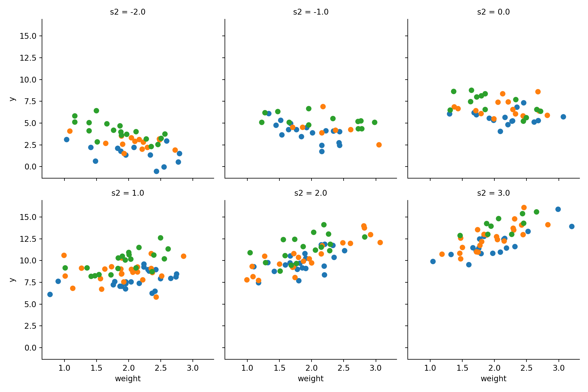
We can see that higher values in s1 have a higher value y, which is obvious because the function is monotonic growing in s1. Moreover our correlations between price and size and weight and size are obvious.
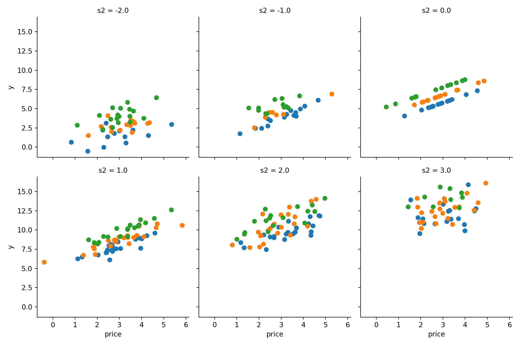
g = sns.FacetGrid(data, col='s2', hue='s1', col_wrap=3, height=3.5);
g = g.map_dataframe(plt.scatter, 'price', 'y');
plt.show()
A toy example how it would appear in (a kind) reality 🔗
But now the problem: we do not know the features s1, s2 and s3, but only the product ids & supplier ids. To simulate how this dataset would appear in the wild let us introduce a hash function that we will use to obfuscate our unmeasurable features and generate some product and supplier ids.
import hashlib

def generate_hash(*args):
    s = '_'.join([str(x) for x in args])
    return hashlib.md5(s.encode()).hexdigest()[-4:]

generate_hash('a', 2)
## '5724'
generate_hash(123)
## '4b70'
generate_hash('a', 2)
## '5724'
We can now generate our data with obfuscated properties, replaced by product ids:
def generate_data(n, s1_bins, s2_bins, s3_bins):
    data = generate_secret_data(n, s1_bins, s2_bins, s3_bins)

    # generate product id from (s1, s3), supplier id from (s2, s3)
    data['product_id'] = data.apply(lambda row: generate_hash(row['s1'], row['s3']), axis=1)
    data['supplier_id'] = data.apply(lambda row: generate_hash(row['s2'], row['s3']), axis=1)

    # drop  secret features
    data = data.drop(['s1', 's2', 's3'], axis=1)

    return data[['product_id', 'supplier_id', 'price', 'weight', 'y']]

data = generate_data(n=300, s1_bins=4, s2_bins=1, s3_bins=2)
data.head(10)
##   product_id supplier_id  price  weight      y
## 0       7235        a154  2.228   2.287  4.470
## 1       9cb6        a154  3.629   2.516  8.986
## 2       3c7e        0aad  3.968   1.149  8.641
## 3       4184        0aad  3.671   2.044  7.791
## 4       4184        0aad  3.637   1.585  7.528
## 5       38f9        a154  1.780   1.661  4.709
## 6       7235        a154  3.841   2.201  6.040
## 7       efa0        0aad  2.773   2.055  4.899
## 8       4184        0aad  3.094   1.822  7.104
## 9       4184        0aad  4.080   2.826  8.591
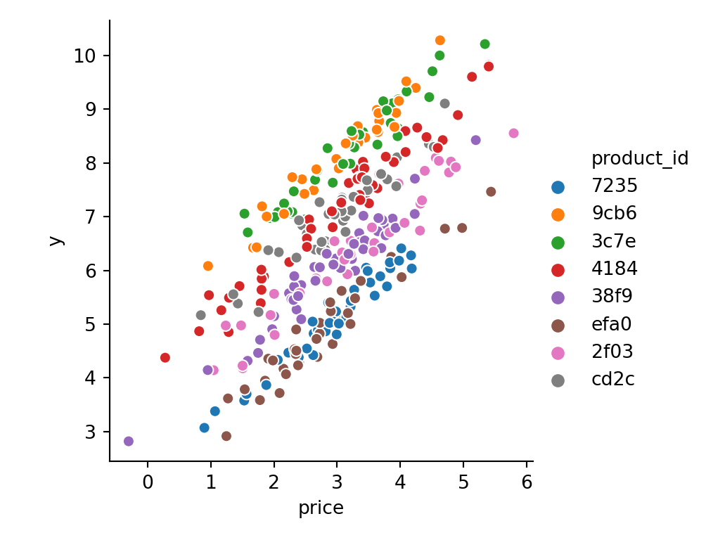
We still see that different products tend to have different values, but we cannot easily compute the size value from the product id any more:
sns.relplot(
    x='price',
    y='y',
    hue='product_id',
    sizes=(40, 400),
    alpha=1,
    height=4,
    data=data
);

plt.show()
Let us generate a bigger dataset now. To be able to fairly compare our embedding model with a more naive baseline, and to be able to validate our approach, we will assume rather small values for our categorical cardinalities S1_BINS, S2_BINS, S3_BINS. If S1_BINS, S2_BINS, S3_BINS >> 10000 the benchmark models will run into memory issues and will perform poorly.
from sklearn.model_selection import train_test_split

N = 100000
S1_BINS = 30
S2_BINS = 3
S3_BINS = 50
data = generate_data(n=N, s1_bins=S1_BINS, s2_bins=S2_BINS, s3_bins=S3_BINS)

data.describe()

# cardinality of c1 is approx S1_BINS * S3_BINS,
# c2 is approx. S2_BINS * S3_BINS
##             price      weight           y
## count  100000.000  100000.000  100000.000
## mean        3.005       2.002      17.404
## std         0.997       0.502       8.883
## min        -1.052      -0.232      -2.123
## 25%         2.332       1.664       9.924
## 50%         3.004       2.002      17.413
## 75%         3.676       2.341      24.887
## max         7.571       4.114      38.641
data.describe(include='object')
##        product_id supplier_id
## count      100000      100000
## unique       1479         149
## top          8851        0d98
## freq          151        1376
We will now split the data into features and response, and train and test.
x = data[['product_id', 'supplier_id', 'price', 'weight']]
y = data[['y']]
x_train, x_test, y_train, y_test = train_test_split(x, y, random_state=456)
Building benchmark models: naive and baseline 🔗
Let us first assemble a very naive linear model, which performs quite poorly and only tries to estimate size from price and weight:
from sklearn.linear_model import LinearRegression
from sklearn.metrics import mean_squared_error, mean_absolute_error

naive_model = LinearRegression()
naive_model.fit(x_train[['price', 'weight']], y_train);

y_pred_naive = naive_model.predict(x_test[['price', 'weight']])

mean_squared_error(y_test, y_pred_naive)
## 77.63320758421973
mean_absolute_error(y_test, y_pred_naive)
## 7.586725358761727
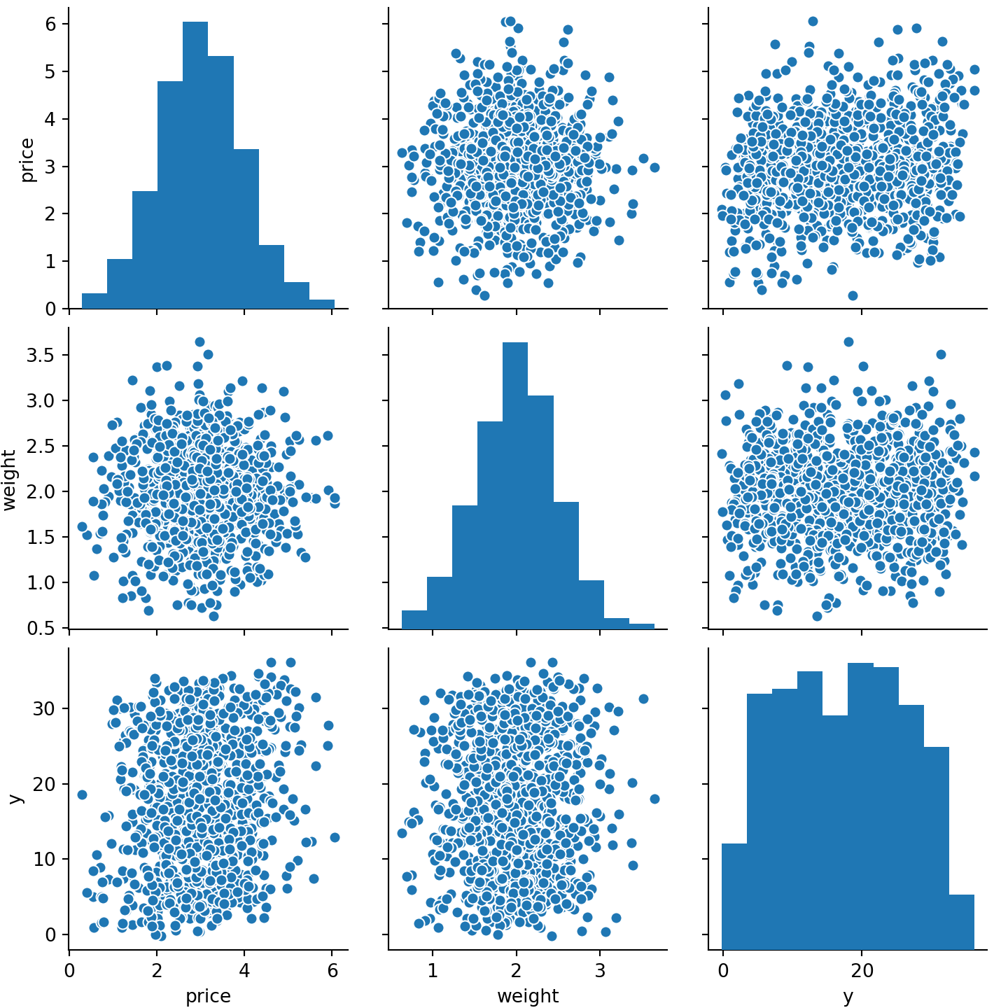
The bad performance close to the overall variance of the response is obvious if we look at the correlations between price and weight and the response size, ignoring the ids:
sns.pairplot(data[['price', 'weight', 'y']].sample(1000))
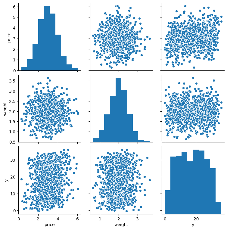
plt.show()
For a better benchmark we can one-hot-encode the categorical features and standardize the numeric data, using the sklearns ColumnTransformer to apply these transformations to different columns. Due to the amount of features we will use Ridge regression instead of normal linear regression to keep the coefficients small (but non-zero, unlike with Lasso, which would lead to losing information about specific classes). Alternatively you can also use KBinsDiscretizer, which did not perform much better for me.
from sklearn.preprocessing import OneHotEncoder, StandardScaler
from sklearn.compose import ColumnTransformer

def create_one_hot_preprocessor():
    return ColumnTransformer([
        ('one_hot_encoder', OneHotEncoder(sparse=False, handle_unknown='ignore'), ['product_id', 'supplier_id']),
        ('standard_scaler', StandardScaler(), ['price', 'weight'])]
    )
The one hot preprocessor spreads the features to columns and makes the data wide, additionally the numerical features get standardized to zero mean and unit variance:
sample_data = data.head(5)
sample_data
##   product_id supplier_id  price  weight       y
## 0       d4b7        c16d  1.846   1.496  25.981
## 1       9674        1030  2.308   1.972  26.213
## 2       78f6        ad7f  3.116   2.464  19.774
## 3       ac69        95a8  1.747   2.188   5.544
## 4       448c        a8b7  1.708   2.129  15.533
one_hot_preprocessor = create_one_hot_preprocessor()
one_hot_preprocessor.fit_transform(sample_data)
## array([[ 0.   ,  0.   ,  0.   ,  0.   ,  1.   ,  0.   ,  0.   ,  0.   ,
##          0.   ,  1.   , -0.563, -1.734],
##        [ 0.   ,  0.   ,  1.   ,  0.   ,  0.   ,  1.   ,  0.   ,  0.   ,
##          0.   ,  0.   ,  0.307, -0.245],
##        [ 0.   ,  1.   ,  0.   ,  0.   ,  0.   ,  0.   ,  0.   ,  0.   ,
##          1.   ,  0.   ,  1.83 ,  1.297],
##        [ 0.   ,  0.   ,  0.   ,  1.   ,  0.   ,  0.   ,  1.   ,  0.   ,
##          0.   ,  0.   , -0.75 ,  0.433],
##        [ 1.   ,  0.   ,  0.   ,  0.   ,  0.   ,  0.   ,  0.   ,  1.   ,
##          0.   ,  0.   , -0.824,  0.249]])
from sklearn.pipeline import Pipeline
from sklearn.linear_model import Ridge

baseline_pipeline = Pipeline(steps=[
    ('preprocessor', create_one_hot_preprocessor()),
    ('model', Ridge())
])

baseline_pipeline.fit(x_train, y_train);
y_pred_baseline = baseline_pipeline.predict(x_test)

mean_squared_error(y_test, y_pred_baseline)
## 0.34772562548572533
mean_absolute_error(y_test, y_pred_baseline)
## 0.387767589378646
Building a neural net with embedding layers, including preprocessing and unknown category handling 🔗
Now let us build a neural net model with embedding layers for our categoricals. To feed them to the embedding layer we need to map the categorical variables to numerical sequences first, i.e. integers from the intervals [0, #supplier ids] resp. [0, #product ids].
Since sklearns OrdinalEncoder cannot handle unknown values as of now, we need to improvise. Unknown categories might occur when splitting test data randomly or seeing new data in the wild during prediction time. Therefore we have to use a simple implementation (working with dataframes instead of arrays, not optimized for speed) of an encoder which can handle unknown values: we essentially use an ordered dictionary as a hashmap to map values to positive integer ranges, where unknown values will get mapped to 0 (we need to map to non-negative values to conform with the embedding layer later on).
from sklearn.base import BaseEstimator, TransformerMixin
from pandas.api.types import is_string_dtype
from collections import OrderedDict

class ColumnEncoder(BaseEstimator, TransformerMixin):
    def __init__(self):
        self.columns = None
        self.maps = dict()

    def transform(self, X):
        X_copy = X.copy()
        for col in self.columns:
            # encode value x of col via dict entry self.maps[col][x]+1 if present, otherwise 0
            X_copy.loc[:,col] = X_copy.loc[:,col].apply(lambda x: self.maps[col].get(x, -1)+1)
        return X_copy

    def inverse_transform(self, X):
        X_copy = X.copy()
        for col in self.columns:
            values = list(self.maps[col].keys())
            # find value in ordered list and map out of range values to None
            X_copy.loc[:,col] = [values[i-1] if 0<i<=len(values) else None for i in X_copy[col]]
        return X_copy

    def fit(self, X, y=None):
        # only apply to string type columns
        self.columns = [col for col in X.columns if is_string_dtype(X[col])]
        for col in self.columns:
            self.maps[col] = OrderedDict({value: num for num, value in enumerate(sorted(set(X[col])))})
        return self
The encoder can now encode and decode our data:
ce = ColumnEncoder()

ce.fit_transform(x_train)
##        product_id  supplier_id  price  weight
## 17414         941          104  2.536   1.885
## 54089         330          131  3.700   1.847
## 84350         960          122  3.517   2.341
## 68797         423           77  4.942   1.461
## 50994         617          138  4.276   1.272
## ...           ...          ...    ...     ...
## 55338         218          118  2.427   2.180
## 92761         528           10  1.705   1.368
## 48811         399           67  3.579   1.938
## 66149         531          126  2.216   2.997
## 30619        1141           67  1.479   1.888
##
## [75000 rows x 4 columns]
ce.inverse_transform(ce.transform(x_train))
##       product_id supplier_id  price  weight
## 17414       a61d        b498  2.536   1.885
## 54089       36e6        e41f  3.700   1.847
## 84350       a868        d574  3.517   2.341
## 68797       4868        80cf  4.942   1.461
## 50994       69f3        eb54  4.276   1.272
## ...          ...         ...    ...     ...
## 55338       2429        cc4a  2.427   2.180
## 92761       5c02        0ec5  1.705   1.368
## 48811       426c        7a7d  3.579   1.938
## 66149       5d45        dc6f  2.216   2.997
## 30619       c73d        7a7d  1.479   1.888
##
## [75000 rows x 4 columns]
x_train.equals(ce.inverse_transform(ce.transform(x_train)))
## True
It can also handle unknown data by mapping it to the zero-category:
unknown_data = pd.DataFrame({
    'product_id': ['!§$%&/()'],
    'supplier_id': ['abcdefg'],
    'price': [10],
    'weight': [20],
  })

ce.transform(unknown_data)
##    product_id  supplier_id  price  weight
## 0           0            0     10      20
ce.inverse_transform(ce.transform(unknown_data))
##   product_id supplier_id  price  weight
## 0       None        None     10      20
To feed the data to the model we need to split the input to pass it to different layers, essentially into X = [X_embedding1, X_embedding2, X_other]. We can do this using a transformer again, this time working with np.arrays, since the StandardScaler returns arrays:
class EmbeddingTransformer(BaseEstimator, TransformerMixin):
    def __init__(self, cols):
        self.cols = cols

    def fit(self, X, y=None):
        self.other_cols = [col for col in range(X.shape[1]) if col not in self.cols]
        return self

    def transform(self, X):
        if len(self.cols) == 0:
            return X
        if isinstance(X, pd.DataFrame):
            X = X.to_numpy()
        X_new = [X[:,[col]] for col in self.cols]
        X_new.append(X[:,self.other_cols])
        return X_new
emb = EmbeddingTransformer(cols=[0, 1])
emb.fit_transform(x_train.head(5))
## [array([['a61d'],
##        ['36e6'],
##        ['a868'],
##        ['4868'],
##        ['69f3']], dtype=object), array([['b498'],
##        ['e41f'],
##        ['d574'],
##        ['80cf'],
##        ['eb54']], dtype=object), array([[2.5360678952988436, 1.8849677601403312],
##        [3.699501628053666, 1.8469279753798342],
##        [3.5168780519630527, 2.340554963373134],
##        [4.941651644756232, 1.4606898248596456],
##        [4.27624682317603, 1.2715509823965785]], dtype=object)]
Let’s combine those two now, and fit the preprocessor with the training data to encode the categories, perform the scaling and bring it into the right format:
def create_embedding_preprocessor():
  encoding_preprocessor = ColumnTransformer([
      ('column_encoder', ColumnEncoder(), ['product_id', 'supplier_id']),
      ('standard_scaler', StandardScaler(), ['price', 'weight'])
  ])

  embedding_preprocessor = Pipeline(steps=[
      ('encoding_preprocessor', encoding_preprocessor),
      # careful here, column order matters:
      ('embedding_transformer', EmbeddingTransformer(cols=[0, 1])),
  ])

  return embedding_preprocessor

embedding_preprocessor = create_embedding_preprocessor()
embedding_preprocessor.fit(x_train);
If we feed this data to the model now it will not be able to learn anything reasonable for unknown categories, i.e. categories that did not exist in the training data x_train when we did the fit. So once we try to make predictions for those we might receive unreasonable estimates.
One way to tackle this out-of-vocabulary problem is to set some random training observations to unknown categories. Therefore during the training of the model, the transformation will encode these with 0, which is the token for unknowns, and it will allow the model to learn something close to the mean for unknown categories. With more domain knowledge we could also pick any other category as default, instead of sampling at random.
The cardinalities of our categorical variables product_id and supplier_id can be computed in the following way, and we will need them once we build our embedding layers.
# vocab sizes
C1_SIZE = x_train['product_id'].nunique()
C2_SIZE = x_train['supplier_id'].nunique()

x_train = x_train.copy()
n = x_train.shape[0]

idx1 = np_random_state.randint(0, n, int(n / C1_SIZE))
x_train.iloc[idx1,0] = '(unknown)'

idx2 = np_random_state.randint(0, n, int(n / C2_SIZE))
x_train.iloc[idx2,1] = '(unknown)'

x_train.sample(10, random_state=1234)
##       product_id supplier_id  price  weight
## 17547       7340        6d30  1.478   1.128
## 67802       4849        f7d5  3.699   1.840
## 17802       de88        55a0  3.011   2.306
## 36366       0912        1d0d  2.453   2.529
## 27847       f254        56a6  2.303   2.762
## 19006       2296   (unknown)  2.384   1.790
## 34628       798f        5da6  4.362   1.775
## 11069       2499        803f  1.455   1.521
## 69851       cb7e        bfac  3.611   2.039
## 13835       8497        33ab  4.133   1.773
We can now transform the data
x_train_emb = embedding_preprocessor.transform(x_train)
x_test_emb = embedding_preprocessor.transform(x_test)

x_train_emb[0]
## array([[ 941.],
##        [ 330.],
##        [ 960.],
##        ...,
##        [ 399.],
##        [ 531.],
##        [1141.]])
x_train_emb[1]
## array([[104.],
##        [131.],
##        [122.],
##        ...,
##        [ 67.],
##        [126.],
##        [ 67.]])
x_train_emb[2]
## array([[-0.472, -0.234],
##        [ 0.693, -0.309],
##        [ 0.51 ,  0.672],
##        ...,
##        [ 0.572, -0.128],
##        [-0.792,  1.976],
##        [-1.53 , -0.229]])
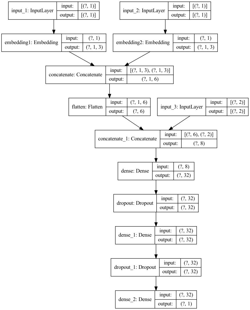
Time to build the neural network! We have 3 inputs (2 embeddings, 1 normal). The embedding inputs are both passed to Embedding layers, flattened and concatenated with the normal inputs. The following hidden layers consist of Dense & Dropout, and are finally activated linearly.
from tensorflow.python.keras.layers import Input, Dense, Reshape, Embedding, concatenate, Dropout, Flatten
from tensorflow.python.keras.layers.merge import Dot
from tensorflow.python.keras.preprocessing import sequence
from tensorflow.python.keras import Model

def create_model(embedding1_vocab_size = 7,
                 embedding1_dim = 3,
                 embedding2_vocab_size = 7,
                 embedding2_dim = 3):
    embedding1_input = Input((1,))
    embedding1 = Embedding(input_dim=embedding1_vocab_size,
                           output_dim=embedding1_dim,
                           name='embedding1')(embedding1_input)

    embedding2_input = Input((1,))
    embedding2 = Embedding(input_dim=embedding2_vocab_size,
                           output_dim=embedding2_dim,
                           name='embedding2')(embedding2_input)

    flatten = Flatten()(concatenate([embedding1, embedding2]))

    normal_input = Input((2,))

    merged_input = concatenate([flatten, normal_input], axis=-1)

    dense1 = Dense(32, activation='relu')(merged_input)
    dropout1 = Dropout(0.1)(dense1)
    dense2 = Dense(32, activation='relu')(dropout1)
    dropout2 = Dropout(0.1)(dense2)

    output = Dense(1, activation='linear')(dropout2)

    model = Model(inputs=[embedding1_input, embedding2_input, normal_input], outputs=output)
    model.compile(loss='mean_squared_error', optimizer='adam', metrics=['mae'])

    return model
import tensorflow as tf

model = create_model(embedding1_vocab_size=C1_SIZE+1,
                     embedding2_vocab_size=C2_SIZE+1)
## WARNING:tensorflow:From /Users/s.telsemeyer/.virtualenvs/blog_py36_20200223/lib/python3.6/site-packages/tensorflow_core/python/keras/initializers.py:119: calling RandomUniform.__init__ (from tensorflow.python.ops.init_ops) with dtype is deprecated and will be removed in a future version.
## Instructions for updating:
## Call initializer instance with the dtype argument instead of passing it to the constructor
## WARNING:tensorflow:From /Users/s.telsemeyer/.virtualenvs/blog_py36_20200223/lib/python3.6/site-packages/tensorflow_core/python/ops/resource_variable_ops.py:1630: calling BaseResourceVariable.__init__ (from tensorflow.python.ops.resource_variable_ops) with constraint is deprecated and will be removed in a future version.
## Instructions for updating:
## If using Keras pass *_constraint arguments to layers.
tf.keras.utils.plot_model(
    model,
    to_file='img/keras_embeddings_model.png',
    show_shapes=True,
    show_layer_names=True,
)
num_epochs = 50

model.fit(
    x_train_emb,
    y_train,
    validation_data=(x_test_emb, y_test),
    epochs=num_epochs,
    batch_size=64,
    verbose=0,
);
If you see an error like InvalidArgumentError: indices[37,0] = 30 is not in [0, 30) you chose the wrong vocabulary size, which should be the largest index of the embedded values plus 1 according to the docs.
As we can see the model performs comparably good and even better as the baseline linear model for our linear problem, though its true strength it will only come into play when we blow up the space of the categoricals or add non-linearity to the response:
y_pred_emb = model.predict(x_test_emb)

mean_squared_error(y_pred_baseline, y_test)
## 0.34772562548572533
mean_squared_error(y_pred_emb, y_test)
## 0.20731396423590281
mean_absolute_error(y_pred_baseline, y_test)
## 0.387767589378646
mean_absolute_error(y_pred_emb, y_test)
## 0.35031337955625347
We can also extract the weights of the embedding layers (the first row contains the weights for the zero-label):
weights = model.get_layer('embedding1').get_weights()
pd.DataFrame(weights[0]).head(11)
##         0      1      2
## 0   0.136  0.038  0.091
## 1  -0.011  0.102  0.031
## 2  -0.041  0.139 -0.040
## 3   0.237 -0.285  0.494
## 4   0.205 -0.301  0.579
## 5   0.097 -0.065  0.283
## 6   0.035  0.076  0.086
## 7  -0.344  0.345 -0.302
## 8  -0.312  0.340 -0.274
## 9  -0.134  0.184 -0.170
## 10 -0.108  0.094 -0.026
These weights could potentially be persisted somewhere and used as features in other models (pre-trained-embeddings). Looking at the first 10 categories we can see that values from supplier_id with similar responses y have similar weights:
column_encoder = (embedding_preprocessor
  .named_steps['encoding_preprocessor']
  .named_transformers_['column_encoder'])

data_enc = column_encoder.transform(data)

(data_enc
  .sort_values('supplier_id')
  .groupby('supplier_id')
  .agg({'y': np.mean})
  .head(10))
##                   y
## supplier_id
## 1            19.036
## 2            19.212
## 3            17.017
## 4            15.318
## 5            17.554
## 6            19.198
## 7            17.580
## 8            17.638
## 9            16.358
## 10           14.625
Moreover the model performs reasonably for unknown data, since it performs similar as our very naive baseline model and also similar to assuming a simple conditional mean:
unknown_data = pd.DataFrame({
    'product_id': ['!%&/§(645h'],
    'supplier_id': ['foo/bar'],
    'price': [5],
    'weight': [1]
})

np.mean(y_test['y'])

# conditional mean
## 17.403696362314747
idx = x_test['price'].between(4.5, 5.5) & x_test['weight'].between(0.5, 1.5)
np.mean(y_test['y'][idx])

# very naive baseline
## 18.716701011038868
naive_model.predict(unknown_data[['price', 'weight']])

# ridge baseline
## array([[18.905]])
baseline_pipeline.predict(unknown_data)

# embedding model
## array([[18.864]])
model.predict(embedding_preprocessor.transform(unknown_data))
## array([[18.859]], dtype=float32)
Wrap up 🔗
We have seen how we can leverage embedding layers to encode high cardinality categorical variables, and depending on the cardinality we can also play around with the dimension of our dense feature space for better performance. The price for this is a much more complicated model opposed to running a classical ML approach with one-hot-encoding. If a classical model is preferred, the category weights can be extracted from the embedding layer and used as features in a simpler model, therefore replacing the one-hot-encoding step.