This post is a short intro on combining different machine learning models for practical purposes, to find a good balance between their advantages and disadvantages. In our case we will ensemble a random forest, a very powerful non-linear, non-parametric tree-based allrounder, with a classical linear regression model, a model that is very easy to interpret and can be verified using domain knowledge.
For many problems gradient boosting or random forests are the go-to-model. They often outperform many other models as they are able to learn almost any linear or non-linear relationship. Nevertheless one of the disadvantages of tree models is that they do not handle new data very well, they often extrapolate poorly - read more on this. For practical purposes that can lead to undesired behaviour, for example when predicting time, distances or cost, which will be outlined in a second.
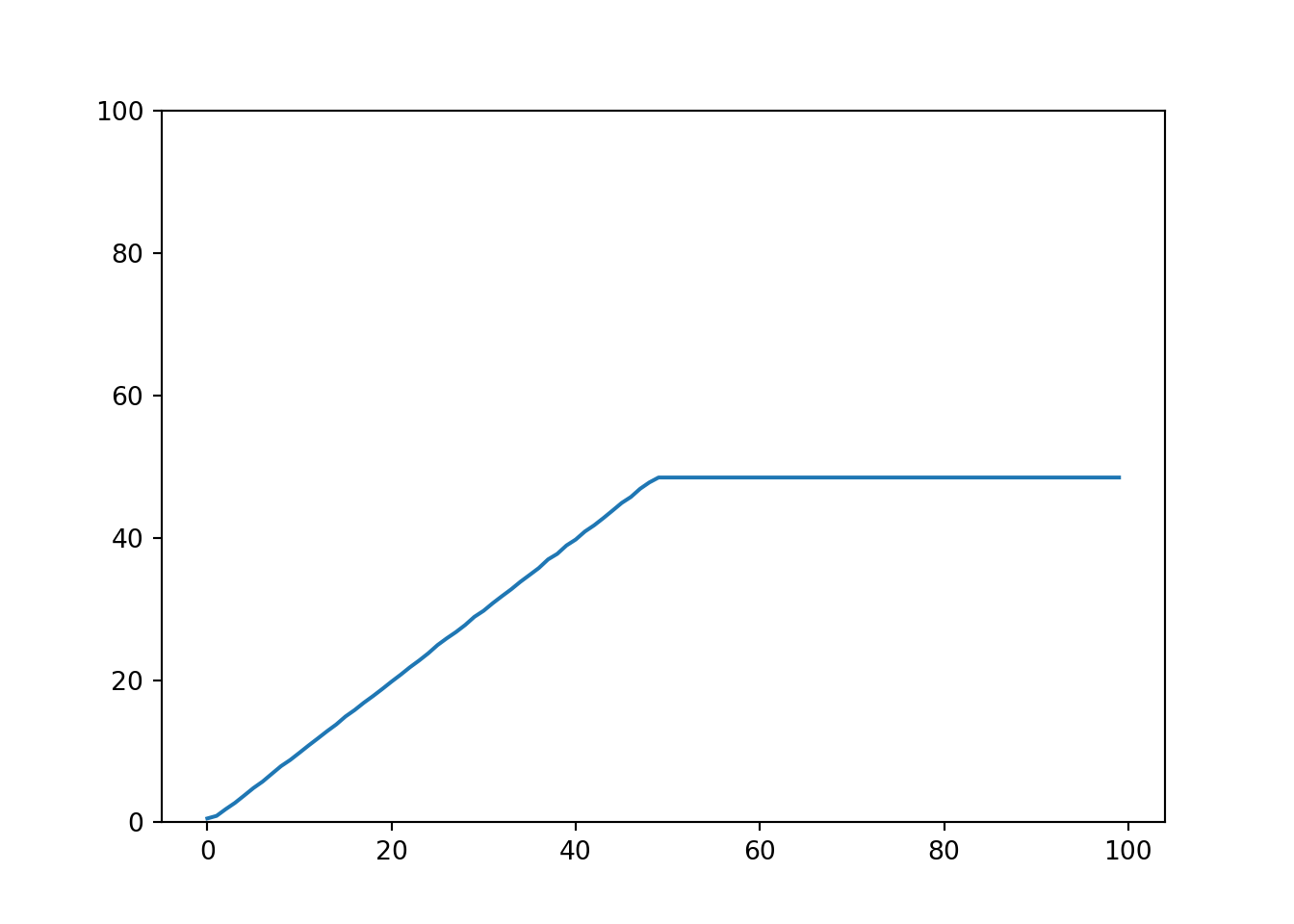
We can quickly verify that the sklearn implementation for random forest models can learn the identity very well for the provided range (0 to 50), but then fails miserably for values out of the training data range.
## Built with python 3.6.15 with following packages:
## pandas==0.25.3
## seaborn==0.9.0
## numpy==1.16.5
## scikit-learn==0.22
## mock==4.0.3
import numpy as np
import matplotlib.pyplot as plt
import seaborn as sns

from sklearn.ensemble import RandomForestRegressor


model = RandomForestRegressor()

X = np.arange(0, 100).reshape(-1, 1)
y = np.arange(0, 100)

# train on [0, 50]
model.fit(X[:50], y[:50]);
# predict for [0, 100]
plt.ylim(0, 100);
sns.lineplot(X.reshape(-1,), model.predict(X));
plt.show()
In contrast to tree models, linear models handle new data differently. They can very easily extrapolate predictions, but of course with the drawback of learning only linear relationships. Moreover linear models allow an easy interpretation, simply by looking at the regression coefficients we can actually compare it to domain knowledge, and practically verify it.
For some regression problems it therefore makes sense to combine both approaches, which we can elaborate with an example: Let’s assume we want to estimate travel time with respect to travel distance for different vehicles, using historic data (a dataset containing the vehicle type, distances and the travel time). We might consider using a linear or a non-linear model, also depending on our expectations. If we aim to estimate travel time for bikes, an increase in distance leads to proportional change in time (if you ride a bike twice as long you can probably travel twice the distance). If we train a linear model it will be a good fit, and the coefficient expresses the proportionality between distance and time.
But a drawback of a linear model is that it could have problems learning the relationship of time versus distance for other vehicle types, like cars. If the travel distance by car increases we might be able to take highways, opposed to the shorter distances, so the increase in travel time might not be linearly proportional any more. In this case a non-linear model may perform better (alternatively we could also transform our input features). However, if we train a non-linear tree model on observed traveled car distances, it will perform poorly on new data, i.e. unseen distances: if our training data only contains car trips up to 100 kilometers, an estimate for 200 kilometers will be very bad, whereas the linear model will still provide a good, extrapolated estimate.
To tackle this we could support the tree model with a linear model in the following way: if the prediction of the tree model is too far away from the prediction of our baseline linear model, we default to the linear model prediction. So for our example: if the non-linear model prediction for a 200 kilometer car ride is 2 hours (because it has only seen car rides up to 2 hours), but the linear model prediction is 3 hours, we default to the 3 hours. Whereas if the prediction of the non-linear model is not too far away (say less than 25%) from the validation prediction of the linear model, we stick to it (as we expect it to perform better in general).
Writing your own combined estimator 🔗
In sklearn we could implement this in the following way,
by creating our own estimator. Be advised that this first implementation does not comply with the sklearn API standards yet - we will improve this version at the end of this post according to the interface.
from sklearn.base import BaseEstimator, RegressorMixin
from sklearn.ensemble import RandomForestRegressor
from sklearn.linear_model import LinearRegression


class CombinedRegressor(BaseEstimator, RegressorMixin):
    def __init__(self, lower=0.75, upper=1.25):
        self.base_regressor = RandomForestRegressor()
        self.backup_regressor = LinearRegression()

        self.lower = lower
        self.upper = upper

    def fit(self, X, y):
        self.base_regressor.fit(X, y)
        self.backup_regressor.fit(X, y)
        return self

    def predict(self, X, y=None):
        y_base = self.base_regressor.predict(X)
        y_backup = self.backup_regressor.predict(X)
        y_pred = np.where((self.lower * y_backup <= y_base) & (y_base <= self.upper * y_backup),
                          y_base,
                          y_backup)
        return y_pred
We simply fit two estimators, and predict using two estimators. We can then compare both predictions and adjust our prediction accordingly. We will take the tree model prediction if it is within a certain range of the linear prediction. Alternatively to comparing both models and picking the more reasonable prediction, we can also take the average of both predictions or blend them differently. Moreover we could optimize the parameters upper and lower using grid search (for this we will need to implement some further methods like get_params and set_params).
Let us generate some sample data using the non-linear function f(x)=x+sqrt(x)+rnorm(0, 3) to evaluate the model:
import pandas as pd


def f(x):
    if isinstance(x, int):
        return np.sqrt(x) + np.random.normal(0, 3)
    else:
        return np.sqrt(x) + np.random.normal(0, 3, len(x))

def generate_data(n=100, x_max=100):
    x = np.random.uniform(0, x_max, n)
    return pd.DataFrame.from_records({'x': x}), f(x)
We can now train three different models: RandomForestRegressor, LinearRegression and our custom CombinedRegressor on our small sample dataset.
models = {
    "tree": RandomForestRegressor(),
    "linear": LinearRegression(),
    "combined": CombinedRegressor()
}
from sklearn.metrics import mean_absolute_error


np.random.seed(100)
X, y = generate_data(n=100)

for model_name, model in models.items():
    print(f'Training {model_name} model.')
    model.fit(X, y);
    print(f'Training score: {model.score(X, y)}')
    print(f'In-sample MAE: {mean_absolute_error(y, model.predict(X))} \n')
## Training tree model.
## RandomForestRegressor(bootstrap=True, ccp_alpha=0.0, criterion='mse',
##                       max_depth=None, max_features='auto', max_leaf_nodes=None,
##                       max_samples=None, min_impurity_decrease=0.0,
##                       min_impurity_split=None, min_samples_leaf=1,
##                       min_samples_split=2, min_weight_fraction_leaf=0.0,
##                       n_estimators=100, n_jobs=None, oob_score=False,
##                       random_state=None, verbose=0, warm_start=False)
## Training score: 0.862081608711054
## In-sample MAE: 1.081361379476639
##
## Training linear model.
## LinearRegression(copy_X=True, fit_intercept=True, n_jobs=None, normalize=False)
## Training score: 0.28917115492576073
## In-sample MAE: 2.586843328406717
##
## Training combined model.
## CombinedRegressor(lower=0.75, upper=1.25)
## Training score: 0.35418433030406293
## In-sample MAE: 2.3593815648352554
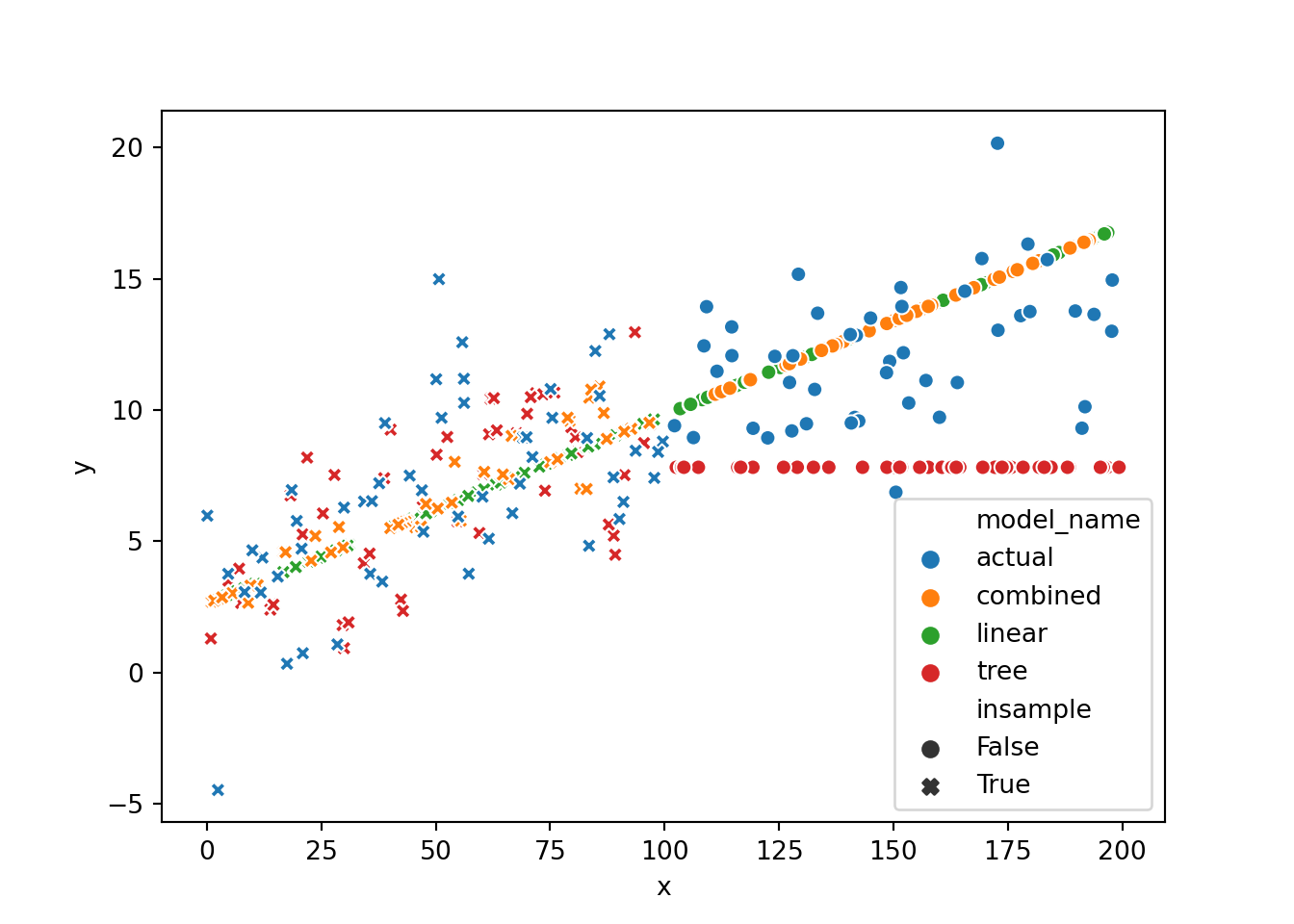
If we look at plots of all three model predictions and the true values we can quickly see the initially discussed problem: the tree model cannot really extrapolate
As expected the random forest model performs best in terms of in-sample mean absolute error. Now if we evaluate out-of-sample (150 opposed to the maximum of 100 in the training data) things look different:
np.random.seed(101)

x = [150]
X_new, y_new = pd.DataFrame({'x': x}), f(x)

for model_name, model in models.items():
    y_pred = model.predict(X_new)
    print(f'Testing {model_name} model.')
    print(f'y_new: {y_new}, y_pred: {y_pred}')
    print(f'Test MAE: {mean_absolute_error(y_new, y_pred)} \n')
## Testing tree model.
## y_new: [20.36799823], y_pred: [7.81515835]
## Test MAE: 12.552839880512696
##
## Testing linear model.
## y_new: [20.36799823], y_pred: [13.39757247]
## Test MAE: 6.970425764867624
##
## Testing combined model.
## y_new: [20.36799823], y_pred: [13.39757247]
## Test MAE: 6.970425764867624
The tree model makes a bad job due to the incapability of extrapolation, the linear model does a better job, and therefore the ensembled model that is backed up by the linear regression. At the same time it will still perform good in-sample, and it will perform decent (better than the tree model only, worse than the linear regression) if we increase the range drastically:
np.random.seed(102)

X_new, y_new = generate_data(n=100, x_max=200)

for model_name, model in models.items():
    y_pred = model.predict(X_new)
    print(f'Testing {model_name} model.')
    print(f'Test MAE: {mean_absolute_error(y_new, y_pred)} \n')
## Testing tree model.
## Test MAE: 3.67092130330585
##
## Testing linear model.
## Test MAE: 2.5770058863460985
##
## Testing combined model.
## Test MAE: 2.6143623109839984
We can also plot the individual predictions on some random data (both in and out of training sample) and quickly see the initially discussed problem of previously unseen x-values and the tree model, which flattens out. The linear model continues with the trend, and the combined version has an unpleasant bump but at least follows the trend once the tree model deviates too much.
Sklearn compatibility 🔗
If we want to achieve full sklearn compatiblity (model selection, pipelines, etc.) and also use sklearn’s onboard testing utilities we have to do some modifications to the estimator:
- we need to add the setters and getters for parameters (we use sklearn’s convention to prefix the
parameters with the name and two underscores, i.e.
base_regressor__some_param) - consistent handling of the random state
This can be achieved in the following way:
import numpy as np

from sklearn.base import BaseEstimator, RegressorMixin
from sklearn.ensemble import RandomForestRegressor
from sklearn.linear_model import LinearRegression


class CombinedRegressor(BaseEstimator, RegressorMixin):
    def __init__(self,
                 base_regressor=RandomForestRegressor,
                 backup_regressor=LinearRegression,
                 lower=0.1,
                 upper=1.9,
                 random_state=None,
                 **kwargs):
        self.base_regressor = base_regressor()
        self.backup_regressor = backup_regressor()

        self.set_random_state(random_state)

        self.lower = lower
        self.upper = upper

        self.set_params(**kwargs)

    def fit(self, X, y):
        self.base_regressor.fit(X, y)
        self.backup_regressor.fit(X, y)
        return self

    def predict(self, X, y=None):
        y_base = self.base_regressor.predict(X)
        y_backup = self.backup_regressor.predict(X)
        y_pred = np.where((self.lower * y_backup <= y_base) & (y_base <= self.upper * y_backup),
                          y_base,
                          y_backup)
        return y_pred

    def __repr__(self):
        # not as good as sklearn pretty printing,
        # but shows updated params of subestimator
        return f'CombinedRegressor({self.get_params()})'

    def get_params(self, deep=False, **kwargs):
        base_regressor_params = self.base_regressor.get_params(**kwargs)
        # remove random state as it should be a global param of the estimator
        base_regressor_params.pop('random_state', None)
        base_regressor_params = {'base_regressor__' + key: value
                                 for key, value
                                 in base_regressor_params.items()}

        backup_regressor_params = self.backup_regressor.get_params(**kwargs)
        backup_regressor_params.pop('random_state', None)
        backup_regressor_params = {'backup_regressor__' + key: value
                                   for key, value
                                   in backup_regressor_params.items()}

        own_params = {
            'lower': self.lower,
            'upper': self.upper,
            'random_state': self.random_state
        }

        params = {**own_params,
                  **base_regressor_params,
                  **backup_regressor_params,
                 }

        if deep:
            params['base_regressor'] = self.base_regressor
            params['backup_regressor'] = self.backup_regressor
        return params

    def set_random_state(self, value):
        self.random_state = value
        if 'random_state' in self.base_regressor.get_params().keys():
            self.base_regressor.set_params(random_state=value)
        # linear reg does not have random state, but just in case..
        if 'random_state' in self.backup_regressor.get_params().keys():
            self.backup_regressor.set_params(random_state=value)

    def set_params(self, **params):
        for key, value in params.items():
            if key.startswith('base_regressor__'):
                trunc_key = {key[len('base_regressor__'):]: value}
                self.base_regressor.set_params(**trunc_key)
            elif key.startswith('backup_regressor__'):
                trunc_key = {key[len('backup_regressor__'):]: value}
                self.backup_regressor.set_params(**trunc_key)
            elif key == 'random_state':
                self.set_random_state(value)
            else:
                # try to fetch old value first to raise AttributeError
                # if not exists
                old_value = getattr(self, key)
                setattr(self, key, value)
        # set_params needs to return self to make gridsearch work
        return self

    def _more_tags(self):
        # no_validation added because validation is happening
        # within built-in sklearn estimators
        return {**self.base_regressor._more_tags(), 'no_validation': True}
We can then run hyperparameter grid search on our custom estimator:
from sklearn.model_selection import GridSearchCV


cv = GridSearchCV(CombinedRegressor(),
                  param_grid={'base_regressor__n_estimators': [50, 100]},
                  verbose=1)

cv.fit(X, y)
## Fitting 5 folds for each of 2 candidates, totalling 10 fits
## GridSearchCV(cv=None, error_score=nan,
##              estimator=CombinedRegressor(backup_regressor__copy_X=True, backup_regressor__fit_intercept=True, backup_regressor__n_jobs=None, backup_regressor__normalize=False, base_regressor__bootstrap=True, base_regressor__ccp_alpha=0.0, base_regressor__criterion='mse', base_regressor__max_depth=None, base_regressor__max_features='...egressor__n_estimators=100, base_regressor__n_jobs=None, base_regressor__oob_score=False, base_regressor__verbose=0, base_regressor__warm_start=False, lower=0.1, random_state=None, upper=1.9),
##              iid='deprecated', n_jobs=None,
##              param_grid={'base_regressor__n_estimators': [50, 100]},
##              pre_dispatch='2*n_jobs', refit=True, return_train_score=False,
##              scoring=None, verbose=1)
##
## [Parallel(n_jobs=1)]: Using backend SequentialBackend with 1 concurrent workers.
## [Parallel(n_jobs=1)]: Done  10 out of  10 | elapsed:    1.1s finished
cv.best_params_
## {'base_regressor__n_estimators': 50}
We can also check our estimator using sklearn.utils.estimator_checks utilities:
from sklearn.utils.estimator_checks import check_estimator

# at once
check_estimator(CombinedRegressor())

# iterate
for estimator, check in check_estimator(CombinedRegressor(), generate_only=True):
    print(f'Running {check}')
    check(estimator)
## Running functools.partial(<function check_no_attributes_set_in_init at 0x12e63e158>, 'CombinedRegressor')
## Running functools.partial(<function check_estimators_dtypes at 0x12e636378>, 'CombinedRegressor')
## Running functools.partial(<function check_fit_score_takes_y at 0x12e636268>, 'CombinedRegressor')
## Running functools.partial(<function check_sample_weights_pandas_series at 0x12e630d08>, 'CombinedRegressor')
## Running functools.partial(<function check_sample_weights_not_an_array at 0x12e630e18>, 'CombinedRegressor')
## Running functools.partial(<function check_sample_weights_list at 0x12e630f28>, 'CombinedRegressor')
## Running functools.partial(<function check_sample_weights_invariance at 0x12e6310d0>, 'CombinedRegressor')
## Running functools.partial(<function check_estimators_fit_returns_self at 0x12e63b2f0>, 'CombinedRegressor')
## Running functools.partial(<function check_estimators_fit_returns_self at 0x12e63b2f0>, 'CombinedRegressor', readonly_memmap=True)
## Running functools.partial(<function check_pipeline_consistency at 0x12e636158>, 'CombinedRegressor')
## Running functools.partial(<function check_estimators_overwrite_params at 0x12e63e048>, 'CombinedRegressor')
## Running functools.partial(<function check_estimator_sparse_data at 0x12e630bf8>, 'CombinedRegressor')
## Running functools.partial(<function check_estimators_pickle at 0x12e6367b8>, 'CombinedRegressor')
## Running functools.partial(<function check_regressors_train at 0x12e63ba60>, 'CombinedRegressor')
## Running functools.partial(<function check_regressors_train at 0x12e63ba60>, 'CombinedRegressor', readonly_memmap=True)
## Running functools.partial(<function check_regressor_data_not_an_array at 0x12e63e488>, 'CombinedRegressor')
## Running functools.partial(<function check_estimators_partial_fit_n_features at 0x12e6368c8>, 'CombinedRegressor')
## Running functools.partial(<function check_regressor_multioutput at 0x12e636ae8>, 'CombinedRegressor')
## Running functools.partial(<function check_regressors_no_decision_function at 0x12e63bb70>, 'CombinedRegressor')
## Running functools.partial(<function check_supervised_y_no_nan at 0x12e62fd90>, 'CombinedRegressor')
## Running functools.partial(<function check_regressors_int at 0x12e63b950>, 'CombinedRegressor')
## Running functools.partial(<function check_estimators_unfitted at 0x12e63b400>, 'CombinedRegressor')
## Running functools.partial(<function check_non_transformer_estimators_n_iter at 0x12e63e8c8>, 'CombinedRegressor')
## Running functools.partial(<function check_fit2d_predict1d at 0x12e631730>, 'CombinedRegressor')
## Running functools.partial(<function check_methods_subset_invariance at 0x12e6318c8>, 'CombinedRegressor')
## Running functools.partial(<function check_fit2d_1sample at 0x12e6319d8>, 'CombinedRegressor')
## Running functools.partial(<function check_fit2d_1feature at 0x12e631ae8>, 'CombinedRegressor')
## Running functools.partial(<function check_fit1d at 0x12e631bf8>, 'CombinedRegressor')
## Running functools.partial(<function check_get_params_invariance at 0x12e63eae8>, 'CombinedRegressor')
## Running functools.partial(<function check_set_params at 0x12e63ebf8>, 'CombinedRegressor')
## Running functools.partial(<function check_dict_unchanged at 0x12e631378>, 'CombinedRegressor')
## Running functools.partial(<function check_dont_overwrite_parameters at 0x12e631620>, 'CombinedRegressor')
## Running functools.partial(<function check_fit_idempotent at 0x12e644048>, 'CombinedRegressor')
In some cases you might not be able to satisfy a specific validation, in this case you could for example mock the return value of that specific check as true:
import mock

from sklearn.utils.estimator_checks import check_estimator


with mock.patch('sklearn.utils.estimator_checks.check_estimators_data_not_an_array', return_value=True) as mock:
    check_estimator(CombinedRegressor())
Wrap up 🔗
This approach can be very helpful if we have one model that works charmingly on a certain set of inputs, but where we lose confidence once the inputs are more exotic. In this case we can guarantee some prediction sanity by using a more transparent (for ex. linear) approach, which we can easily synchronize with domain knowledge and which guarantees a specific behaviour (for ex. extrapolation, proportional increments).
Instead of using a combined estimator we could also use a non-linear model with better extrapolation behaviour, like a neural network. Another alternative would be to add some artificial samples to the training dataset to increase the supported response range.