Remark from May 2022: This post has been updated to work with newer versions of dplyr (1.0.9), multidplyr (0.1.1) and forecast (8.16), but may use some features flagged for deprecation. As of May 2022, there are better alternatives for batch forecasting, like fable in combination with tsibble.
This post will be another quick intro to two magical R packages: purrr and multidplyr.
The first one can be utilized to construct iterations over rows of data frames in a functional way, whereas multidplyr allows to run dataframe mutations in parallel across multiple cores.
For these two packages two work in company, we assemble a dataframe containing a list column containing two time series objects. This will allows us to run time series analysis and prediction using dataframe operations (mutations and summarization), where we will apply functions from the forecast package among others in a rowwise manner. Due to the rowwise nature we will be able to parallelize these operations using multidplyr. Finally we can blend different forecast outputs together and produce a hybrid forecast. For further interest in ensemble forecasting forecastHybrid is recommended.
As sample time series we will use two time series from the fpp2 package: fpp2: Data for “Forecasting: Principles and Practice” (2nd Edition). Extracts from the documentation:
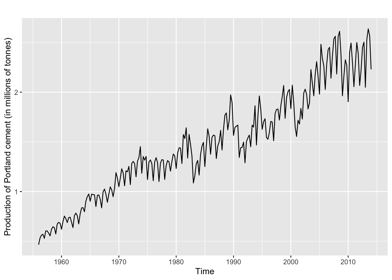
fpp2::qcement: “Total quarterly production of Portland cement in Australia (in millions of tonnes) from 1956:Q1 to 2014:Q1.”fpp2::hyndsight: “Hyndsight is Rob Hyndman’s personal blog at https://robjhyndman.com/hyndsight. This series contains the daily pageviews for one year, beginning 30 April 2014.”
Using a list column we can put these two into a dataframe:
data <- dplyr::tibble(
  id = 1:2,
  y = list(fpp2::qcement, fpp2::hyndsight)
  )
## # A tibble: 2 × 2
##      id y
##   <int> <list>
## 1     1 <ts [233]>
## 2     2 <ts [365]>
data %>%
  dplyr::pull(y) %>%
  .[[1]] %>%
  ggplot2::autoplot() +
  ggplot2::ylab("Production of Portland cement (in millions of tonnes)")
As a first demonstration of the purrr package we will extract the time series frequencies and store them in another column, which will later be used as a forecast horizon and also minimal training period.
The stats::frequency function naturally isn’t vectorized in its first argument x, but purrr::map can overcome this issue. If we expect the output to be a numeric vector (a vector of frequencies) we can more specifically use purrr::map_dbl, and purrr will rather return a numeric vector than a list, or “die trying” (see ?purrr::map).
data <- data %>% dplyr::mutate(h = purrr::map_dbl(.x = y, .f = frequency))
Further we will create a more complicated function which will return a dataframe rather than an vector, which will be nested into the original dataframe after the application of purrr::map. The function partition_ts partitions a time series into sets of training and test data sets: in a first step it will generate a dataframe containing integer representations of possible training period start and end times, as well as the test period start and end times.
In a second step purrr::map2, which allows us to vectorize over two arguments, is applied, such that we can use the window function to extract training and test windows of the time series y. The time series y is not an actual column of the auxiliary dataframe, but sneaked into the map2 function as an additional third argument. Accordingly the train and test time series will be stored in columns train and test: these columns are both lists of S3 time series objects.
partition_ts <- function(y,
                         h = stats::frequency(y),
                         step = stats::frequency(y),
                         min_train = stats::frequency(y)) {
  # extract numeric times
  times <- stats::time(y)

  # extract test start periods from times (start after min_train)
  test_start <- times[seq(min_train + 1, length(times) - h, step)]

  # deltat = 1/freq
  deltat <- stats::deltat(y)

  df <- dplyr::tibble(
    train_start = times[1],
    train_end = test_start - deltat,
    test_start = test_start,
    test_end = test_start + (h-1) * deltat
    )

  df <-
    df %>%
    dplyr::mutate(
      train = purrr::map2(.x = train_start, .y = train_end, .f = window, x = y),
      test = purrr::map2(.x = test_start, .y = test_end, .f = window, x = y)
      )
  return(df)
}
Let’s look at some example before applying it our data dataframe:
partition_ts(ts(1:21, frequency = 7), step = 1)
## # A tibble: 7 × 6
##   train_start train_end test_start test_end train     test
##         <dbl>     <dbl>      <dbl>    <dbl> <list>    <list>
## 1           1      1.86       2        2.86 <ts [7]>  <ts [7]>
## 2           1      2          2.14     3    <ts [8]>  <ts [7]>
## 3           1      2.14       2.29     3.14 <ts [9]>  <ts [7]>
## 4           1      2.29       2.43     3.29 <ts [10]> <ts [7]>
## 5           1      2.43       2.57     3.43 <ts [11]> <ts [7]>
## 6           1      2.57       2.71     3.57 <ts [12]> <ts [7]>
## 7           1      2.71       2.86     3.71 <ts [13]> <ts [7]>
partitions <-
  data %>% dplyr::mutate(partitions = purrr::map2(.x = y, .y = h, .f = partition_ts))
The column partitions of the partitions dataframe now consists of dataframes, which contain sets of time series in its rows. We can unnest this dataframe and make the nested entries rows of the original dataframe data. Using .drop = FALSE we keep tidyr from dropping all other nested columns (in our case: y).
partitions <- partitions %>% tidyr::unnest(partitions, .drop = FALSE)
## Warning: The `.drop` argument of `unnest()` is deprecated as of tidyr 1.0.0.
## All list-columns are now preserved.
## This warning is displayed once every 8 hours.
## Call `lifecycle::last_lifecycle_warnings()` to see where this warning was generated.
Additionally we create a convenience wrapper around some desired univariate forecast functions we plan to use. The function understands two arguments: a time series and a model name, which we can apply to our dataframe of time series in a rowwise manner.
generate_forecast <- function(y, model_name) {
  if (model_name == "zzz") {
    model <- suppressWarnings(forecast::ets(y = y, model = "ZZZ", damped = FALSE,
                                            lambda ="auto", opt.crit = "mse", nmse = 3,
                                            ic = "aic", allow.multiplicative.trend = TRUE))
  } else if (model_name == "zzz_d_14") {
    model <- suppressWarnings(forecast::ets(y = y, model = "ZZZ", damped = TRUE,
                                            lambda = "auto", opt.crit = "mse", nmse = 14,
                                            bounds = "both", ic = "aic",
                                            allow.multiplicative.trend = TRUE))
  } else if (model_name == "tbats") {
    model <- suppressWarnings(forecast::tbats(y))
  } else if (model_name == "mam_d") {
    model <- suppressWarnings(forecast::ets(y, model = "MAM", damped = TRUE))
  } else {
    stop("Model ", model_name, " does not exist.")
  }
  return(model)
}
Let us again quickly look an at example:
generate_forecast(y = ts(101:150 + rnorm(50, 0, sd = 5), frequency = 12),
                  model_name = "tbats")
## BATS(0.761, {0,0}, 1, -)
##
## Call: forecast::tbats(y = y)
##
## Parameters
##   Lambda: 0.761032
##   Alpha: -0.02009984
##   Beta: 0.0001000162
##   Damping Parameter: 1
##
## Seed States:
##            [,1]
## [1,] 42.5091438
## [2,]  0.3098578
## attr(,"lambda")
## [1] 0.7610316
##
## Sigma: 1.610823
## AIC: 368.424
To apply our forecast function to partitions, we create a new column model_name, with the model names unfolded, resulting in a dataframe of nrow(paritions) * length(model_names) rows:
model_names <- c("zzz", "zzz_d_14", "tbats", "mam_d")

partitions <-
  partitions %>%
  dplyr::mutate(model_name = list(model_names)) %>%
  tidyr::unnest(model_name, .drop = FALSE)
## # A tibble: 432 × 10
##       id y              h train_start train_end test_start test_end train  test
##    <int> <list>     <dbl>       <dbl>     <dbl>      <dbl>    <dbl> <list> <lis>
##  1     1 <ts [233]>     4        1956     1957.       1957    1958. <ts>   <ts>
##  2     1 <ts [233]>     4        1956     1957.       1957    1958. <ts>   <ts>
##  3     1 <ts [233]>     4        1956     1957.       1957    1958. <ts>   <ts>
##  4     1 <ts [233]>     4        1956     1957.       1957    1958. <ts>   <ts>
##  5     1 <ts [233]>     4        1956     1958.       1958    1959. <ts>   <ts>
##  6     1 <ts [233]>     4        1956     1958.       1958    1959. <ts>   <ts>
##  7     1 <ts [233]>     4        1956     1958.       1958    1959. <ts>   <ts>
##  8     1 <ts [233]>     4        1956     1958.       1958    1959. <ts>   <ts>
##  9     1 <ts [233]>     4        1956     1959.       1959    1960. <ts>   <ts>
## 10     1 <ts [233]>     4        1956     1959.       1959    1960. <ts>   <ts>
## # … with 422 more rows, and 1 more variable: model_name <chr>
We can now apply our generate_forecast function to each row (i.e. individual training and test set) of the dataframe:
t <- proc.time()

predictions <-
  partitions %>%
  dplyr::mutate(
    model = purrr::map2(.x = train, .y = model_name, .f = generate_forecast),
    prediction = purrr::map2(.x = model, .y = h, .f = predict)
    ) %>%
  dplyr::arrange(id, test_start)

proc.time() - t
##    user  system elapsed
## 516.428   7.048 548.712
This operation can easily be parallelized due to the nature of the rowwise independent mutations. multidplyr allows us to do this with ease: We create a cluster with an assigned number of nodes and ship all needed functions (here: generate_forecast) to the nodes. (The partitioning of the dataframe is done implicitly by multidplyr::partition, but an explicit partitioning can be enforced to run map-reduce like operations.)
t <- proc.time()

cluster <- multidplyr::new_cluster(n = 6)
multidplyr::cluster_copy(cluster, "generate_forecast")

predictions <-
  partitions %>%
  dplyr::mutate(row_number = dplyr::row_number()) %>%
  multidplyr::partition(cluster = cluster) %>%
  dplyr::mutate(
    model = purrr::map2(.x = train, .y = model_name, .f = generate_forecast),
    prediction = purrr::map2(.x = model, .y = h, .f = predict)) %>%
  dplyr::collect() %>%
  dplyr::ungroup() %>%
  dplyr::arrange(id, test_start)

proc.time() - t
##    user  system elapsed
##   0.446   0.203 193.314
In our case we reduced the processing time roughly by a factor of 3, using 6 cores instead of 1. With increasing size of the partitions dataframe the overhead of the master-node setup becomes more irrelevant and higher factors can be achieved. Again using purrr, we can calculate accuracies of our forecasts and extract RMSE and MAE:
predictions <-
  predictions %>%
  dplyr::mutate(
    accuracy = purrr::map2(.x = prediction, .y = test, .f = forecast::accuracy),
    rmse = purrr::map_dbl(.x = accuracy, .f = ~ .x[2, "RMSE"]),
    mae = purrr::map_dbl(.x = accuracy, .f = ~ .x[2, "MAE"])
    )
As we have gathered sets of forecasts from different models for the same time periods, we can now assemble hybrid forecasts by blending different predictions together. We will use the following two functions:
reduce_numericto extract the same elements of a list of prediction objects (mean,fitted, …) and calculate the mean by iterative reduction.blend_predictionsto applyreduce_numericto multiple values of the prediction object and to store the result as aforecast-class object in accordance with theforecastpackage to allow easy plotting.
reduce_numeric <- function(y, value) {
  # extract from lists
  values <- lapply(y, function(x) x[[value]])
  # reduce to mean
  values_avg <- purrr::reduce(values, `+`) / length(values)
  return(values_avg)
}

blend_predictions <- function(predictions) {
  values = list(
    mean = reduce_numeric(predictions, "mean"),
    x = reduce_numeric(predictions, "x"),
    fitted = reduce_numeric(predictions, "fitted"),
    method = "blended ETS models"
    )
  return(structure(values, class = "forecast"))
}
last_item <- nrow(predictions)
blended_prediction <- blend_predictions(list(predictions$prediction[[last_item-1]],
                                             predictions$prediction[[last_item]]))
We can now group the data by time series id and test period start and aggregate the resulting group of predictions to a blended prediction. Join the dataframe of blended forecasts with the test time series we can calculate the accuracies:
blended_predictions <-
  predictions %>%
  dplyr::group_by(id, h, train_start, train_end, test_start, test_end) %>%
  dplyr::summarize(prediction = purrr::map(.x = list(prediction), .f = blend_predictions)) %>%
  dplyr::mutate(model_name = "blended") %>%
  dplyr::ungroup()
## `summarise()` has grouped output by 'id', 'h', 'train_start', 'train_end',
## 'test_start'. You can override using the `.groups` argument.
blended_predictions <-
  partitions %>%
  dplyr::group_by(id, test_start, test_end) %>%
  dplyr::slice(1) %>%
  dplyr::select(id, test_start, test_end, test) %>%
  dplyr::left_join(blended_predictions, ., by = c("id", "test_start", "test_end")) %>%
  dplyr::mutate(
    accuracy = purrr::map2(.x = prediction, .y = test, .f = forecast::accuracy),
    rmse = purrr::map_dbl(.x = accuracy, .f = ~ .x[2, "RMSE"]),
    mae = purrr::map_dbl(.x = accuracy, .f = ~ .x[2, "MAE"])
    )

all_predictions <- dplyr::bind_rows(predictions, blended_predictions)
Its very simple to aggregate metrics using dplyr verbs:
all_predictions %>%
  dplyr::group_by(id, model_name) %>%
  dplyr::summarize_at(dplyr::vars(rmse, mae), list(~ round(mean(.), 3))) %>%
  dplyr::ungroup() %>%
  dplyr::arrange(mae) %>%
  as.data.frame()
##    id model_name    rmse     mae
## 1   1    blended   0.091   0.080
## 2   1      mam_d   0.092   0.081
## 3   1      tbats   0.093   0.081
## 4   1        zzz   0.094   0.082
## 5   1   zzz_d_14   0.093   0.082
## 6   2      tbats 233.037 185.815
## 7   2    blended 235.127 189.240
## 8   2        zzz 234.906 189.459
## 9   2   zzz_d_14 237.109 190.779
## 10  2      mam_d 254.738 209.821
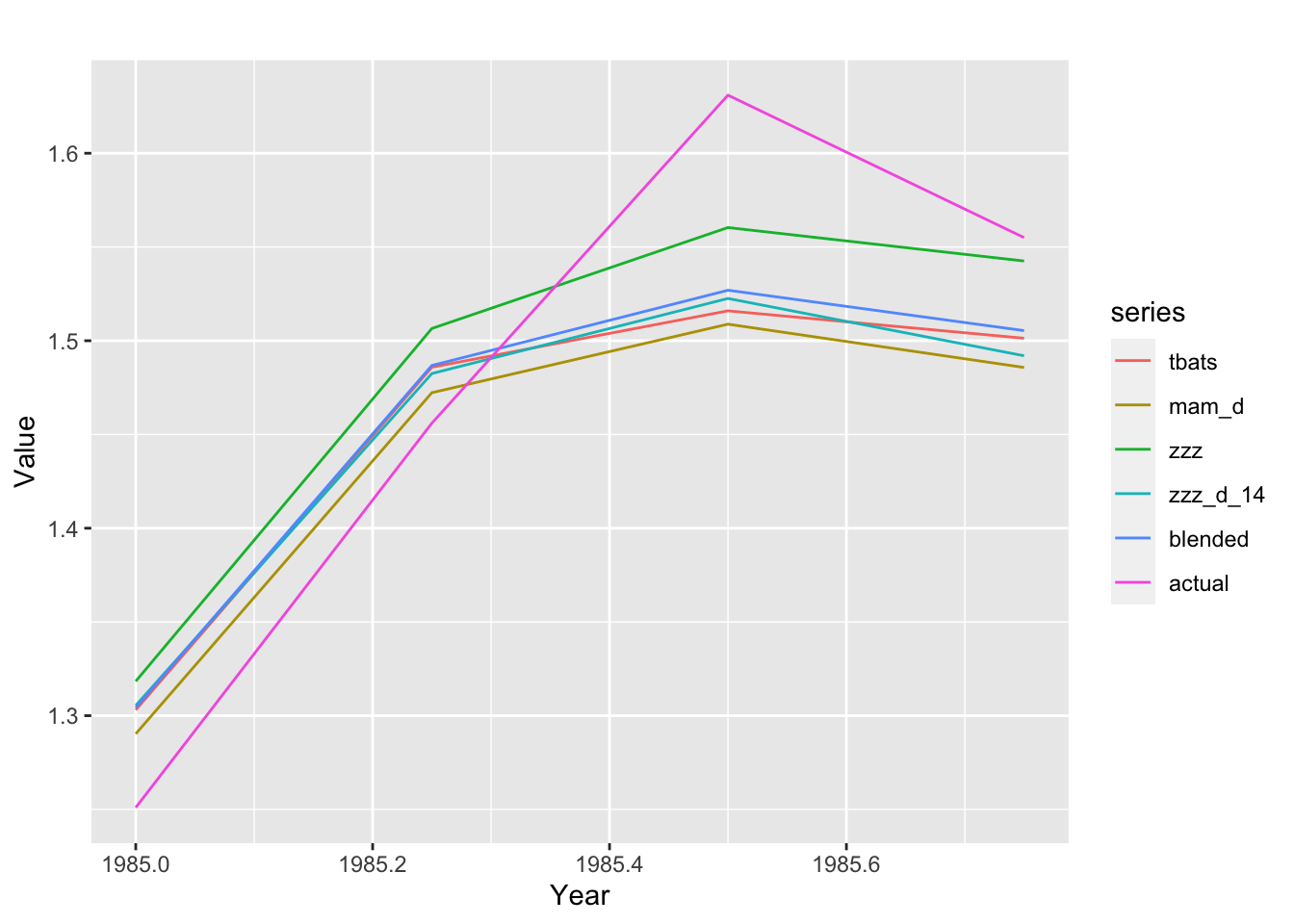
Finally we can extract the point forecasts and the actual data, bind them together to receive a multivariate timeseries, and plot it via ggplot2::autoplot:
predicted_ts <-
  all_predictions %>%
  dplyr::mutate(ts = purrr::map(.x = prediction, .f= "mean")) %>%
  dplyr::select(id, test_start, model_name, ts)

actual_ts <-
  all_predictions %>%
  dplyr::group_by(id, test_start) %>%
  dplyr::slice(1) %>%
  dplyr::ungroup() %>%
  dplyr::mutate(
    model_name = "actual",
    ts = test
    ) %>%
  dplyr::select(id, test_start, model_name, ts)

bind_predictions <- function(predictions, model_names) {
  names(predictions) <- as.list(model_names)
  do.call(cbind, predictions)
}

binded_ts <-
  predicted_ts %>%
  dplyr::bind_rows(actual_ts) %>%
  dplyr::rename(period_start = test_start) %>%
  dplyr::group_by(id, period_start) %>%
  dplyr::summarize(
    mts = purrr::map2(.x = list(ts),
                      .y = list(model_name),
                      .f = bind_predictions)
    ) %>%
  dplyr::ungroup()
## `summarise()` has grouped output by 'id'. You can override using the `.groups`
## argument.
binded_ts %>%
  dplyr::filter(id == 1, period_start == 1985) %>%
  dplyr::pull(mts) %>%
  .[[1]] %>%
  ggplot2::autoplot() + ggplot2::ylab("Value") + ggplot2::xlab("Year")