In this article I want to give a quick intro to two packages: leaflet (2.1.1) and sf (1.0.7). First can be used to draw interactive maps, second to handle geometries dplyr-style, following the simple features specifications. In combination they allow to create simple maps from processed geodata with ease.
Not a prerequisite for the below post, but for further reference on leaflet the illustrated package documentation is suggested. For sf I can recommend the packages vignettes, and for in depth reading also Geocompuation with R. Geospatial computation in R is a popular and quite old topic, but the package sf is quite recent and can be considered as a more convenient successors of the older package sp.
For the ordinary data wrangling the tidyverse package is used, or more specific the well-known dplyr, which works hand in hand with sf. We will also use the famous pipe-operator:
`%>%` <- magrittr::`%>%`
To demonstrate both packages and their interaction we will combine Berlin census data and postcode geometries. The population data is publicly available at the Office for Statistics Berlin-Brandenburg, published as statistical report named A I 5 - hj. The data can be found as a xlsx file (see tab named T14 for the relevant data). I extracted the mentioned tab as a csv file on 2018-04-04 for painless usage.
In the given report missing values are encoded with a dash. One approach to keep proper control over the parsing process and possible failures for this file is to read all columns as characters first and then set all dashes to NA, followed by casting the values to numeric to see if any other parsing problems occur.
postcodes_population <-
  readr::read_delim(
    file = "../../../static/data/postcodes/berlin_census.csv",
    delim = ";",
    col_types = readr::cols(.default = readr::col_character())
    )

postcodes_population <-
  postcodes_population %>%
  dplyr::mutate_at(dplyr::vars(population:female), list(~ dplyr::na_if(x = ., y = "-"))) %>%
  dplyr::mutate_at(dplyr::vars(population:female), as.numeric) %>%
  dplyr::select(postcode, name, population) %>%
  dplyr::arrange(postcode)
## # A tibble: 238 × 3
##    postcode name                 population
##    <chr>    <chr>                     <dbl>
##  1 10115    Mitte                     26274
##  2 10117    Mitte                     15531
##  3 10119    Mitte                     15064
##  4 10119    Pankow                     4606
##  5 10178    Friedrichsh.-Kreuzb.         81
##  6 10178    Mitte                     14385
##  7 10179    Friedrichsh.-Kreuzb.        406
##  8 10179    Mitte                     23564
##  9 10243    Friedrichsh.-Kreuzb.      30655
## 10 10245    Friedrichsh.-Kreuzb.      33509
## # … with 228 more rows
We will only use summarized population data. But if desired the data frame can easily be processed into long format using tidyr::gather for a pleasant further analysis.
We can import all german postcode geometries from a publicly available shapefile (consisting of 3 files following the format’s standard). sf::read_sf (the sp equivalent would be rgdal::readOGR) is a very flexible way to deserialize geometries, as it can read from databases or different kinds of files like shapefiles, geojsons, KML or WKT representations. Once read, the geometries are then stored as sf geometries: a R object consisting of a dataframe containing a feature collection (points, polygons, multipolygons and so on), and some additional metadata, like the used projection and the boundary box:
We can then use dplyr verbs to process the data. It is important to note that the sf package should be loaded to preserve the objects attributes after operations like select or filter (see raised issue here).
postcodes_geometries <- sf::read_sf("../../../static/data/postcodes/shapefile/post_pl.shp")

postcodes_geometries <-
  postcodes_geometries %>%
  # set coordinate reference system to what is stated in the source
  sf::st_set_crs(value = 4326) %>%
  dplyr::select(postcode = PLZ99, geometry)
## Simple feature collection with 8270 features and 1 field
## Geometry type: MULTIPOLYGON
## Dimension:     XY
## Bounding box:  xmin: 5.866286 ymin: 47.2736 xmax: 15.04863 ymax: 55.05826
## Geodetic CRS:  WGS 84
## # A tibble: 8,270 × 2
##    postcode                                                             geometry
##    <chr>                                                      <MULTIPOLYGON [°]>
##  1 01067    (((13.71894 51.076, 13.72122 51.07498, 13.72245 51.07323, 13.7243 5…
##  2 01069    (((13.74984 51.05443, 13.75115 51.05469, 13.75363 51.05537, 13.7571…
##  3 01097    (((13.72758 51.06863, 13.732 51.07026, 13.73651 51.07211, 13.73381 …
##  4 01099    (((13.82016 51.12494, 13.82555 51.12502, 13.82922 51.12535, 13.8291…
##  5 01109    (((13.75954 51.13818, 13.76404 51.13723, 13.76857 51.13533, 13.7799…
##  6 01127    (((13.72008 51.08574, 13.72196 51.08514, 13.72361 51.08428, 13.7249…
##  7 01129    (((13.69849 51.11303, 13.70076 51.11278, 13.70276 51.11421, 13.7029…
##  8 01139    (((13.66451 51.08914, 13.66444 51.0895, 13.66376 51.08989, 13.66321…
##  9 01157    (((13.69622 51.06446, 13.69716 51.06051, 13.69598 51.05796, 13.6937…
## 10 01159    (((13.69598 51.05796, 13.69677 51.05779, 13.69833 51.05746, 13.7045…
## # … with 8,260 more rows
It is easy now to join the geometries with the population information by postcode.
postcodes <- dplyr::right_join(postcodes_geometries, postcodes_population, by = "postcode")
## Simple feature collection with 238 features and 3 fields
## Geometry type: MULTIPOLYGON
## Dimension:     XY
## Bounding box:  xmin: 13.09124 ymin: 52.34047 xmax: 13.80103 ymax: 52.67727
## Geodetic CRS:  WGS 84
## # A tibble: 238 × 4
##    postcode                                            geometry name  population
##    <chr>                                     <MULTIPOLYGON [°]> <chr>      <dbl>
##  1 10115    (((13.3753 52.53998, 13.37701 52.53894, 13.37718 5… Mitte      26274
##  2 10117    (((13.40322 52.52507, 13.40342 52.52394, 13.40187 … Mitte      15531
##  3 10119    (((13.40347 52.53816, 13.40551 52.53685, 13.40567 … Mitte      15064
##  4 10119    (((13.40347 52.53816, 13.40551 52.53685, 13.40567 … Pank…       4606
##  5 10178    (((13.41209 52.53094, 13.41767 52.52957, 13.42305 … Frie…         81
##  6 10178    (((13.41209 52.53094, 13.41767 52.52957, 13.42305 … Mitte      14385
##  7 10179    (((13.43118 52.52072, 13.43042 52.51953, 13.42804 … Frie…        406
##  8 10179    (((13.43118 52.52072, 13.43042 52.51953, 13.42804 … Mitte      23564
##  9 10243    (((13.42845 52.52548, 13.43153 52.52535, 13.4344 5… Frie…      30655
## 10 10245    (((13.45597 52.51645, 13.46093 52.51469, 13.46424 … Frie…      33509
## # … with 228 more rows
To explore the data let us extract some sample rows and display them using leaflet. With just a few lines of code we can create a map, add background tiles and the sample postcode geometries as polygons:
rows <- c(40, 60, 80)
sample_postcodes <- postcodes[rows,]
## Simple feature collection with 3 features and 3 fields
## Geometry type: MULTIPOLYGON
## Dimension:     XY
## Bounding box:  xmin: 13.31064 ymin: 52.47602 xmax: 13.4526 ymax: 52.51623
## Geodetic CRS:  WGS 84
## # A tibble: 3 × 4
##   postcode                                             geometry name  population
##   <chr>                                      <MULTIPOLYGON [°]> <chr>      <dbl>
## 1 10625    (((13.32498 52.51376, 13.3253 52.51303, 13.32383 52… Char…      11864
## 2 10787    (((13.3513 52.51623, 13.35165 52.5159, 13.35192 52.… Mitte       3283
## 3 12043    (((13.42842 52.49003, 13.43328 52.48828, 13.43716 5… Neuk…      15983
map <-
  sample_postcodes %>%
  leaflet::leaflet() %>%
  leaflet::addTiles() %>%
  leaflet::addPolygons()
Although sf offers a lot of different functions for transformations and aggregations of geometries, it is also very easy to extract coordinates as a dataframe using sf::st_coordinates() for straightforward data frame wrangling. Moreover leaflet can also easily interpret lat-long dataframes.
coordinates <-
  sample_postcodes %>%
  sf::st_coordinates() %>%
  dplyr::as_tibble()
another_map <-
  coordinates %>%
  leaflet::leaflet() %>%
  leaflet::addTiles() %>%
  leaflet::addPolygons(lng = ~ X, lat = ~ Y)
Let us now merge the postcode polygons using sf::st_union() and add the resulting outlines to the existing map, red-colored, with slightly thicker outlines.
map <-
  postcodes %>%
  sf::st_union() %>%
  leaflet::addPolylines(map, data = ., weight = 3, color = "red")
In the following we will impute missing postcode names, calculate the postcodes areas and their population density.
postcodes <-
  postcodes %>%
  dplyr::mutate(
    name = dplyr::na_if(name, "Berlin"),
    area = round(sf::st_area(geometry) / 1000 / 1000, 2),
    density = round(as.numeric(population / area))
    )
We will now add all the postcode polygons to a map, colored by density, and add popups with further information which are visible if clicked.
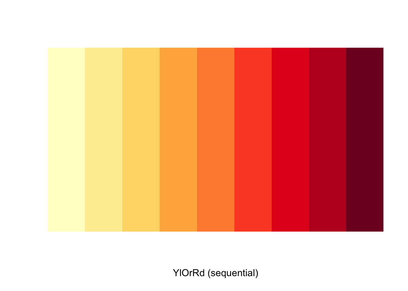
The mapping of values to colors can be done using the package RColorBrewer (other options are available). A list of the package’s color palettes is available via RColorBrewer::display.brewer.all. In our case we will map the population density (more specific: squareroot of the density) to a yellow-to-red palette
RColorBrewer::display.brewer.pal(name = "YlOrRd", n = 9)
Via colorNumeric we can easily define such a function if we specify the domain:
pal <-
  leaflet::colorNumeric(
    palette = "YlOrRd",
    domain = sqrt(postcodes$density),
    na.color = NA
    )
For the popup we can use simple html code and reference data contained in the postcodes object, similar as how it works with ggplot’s aesthetics.
popup_str <- "
<b>Postcode:</b> {postcode} <br>
<b>Name:</b> {name} <br>
<b>Population:</b> {population} <br>
<b>Area:</b> {area} km²<br>
<b>Density:</b> {density} ppl/km² <br>
"

map <-
  postcodes %>%
  leaflet::leaflet() %>%
  leaflet::addTiles() %>%
  leaflet::addPolygons(
    weight = 1,
    color = "black",
    fillOpacity = 0.66,
    group = "Postcodes",
    popup = ~ glue::glue(
      popup_str,
      postcode = postcode,
      name = name,
      population = population,
      area = area,
      density = density
      ),
    fillColor = ~ pal(sqrt(density)),
    highlightOptions = leaflet::highlightOptions(
      opacity = 1,
      color = "black",
      weight = 2,
      bringToFront = TRUE
      )
    ) %>%
  leaflet::addLegend(
    pal = pal,
    values = ~ sqrt(density),
    title = "Density",
    labFormat = leaflet::labelFormat(transform = function(x) x^2),
    na.label = FALSE
    )
We will now demonstrate the function to overlay different features in a map: We can group postcodes by name to create some districts to draw in addition to the individual postcodes.
districts <-
  postcodes %>%
  dplyr::mutate(name = dplyr::coalesce(name, "-")) %>%
  dplyr::group_by(name) %>%
  dplyr::summarize(
    geometry = sf::st_union(geometry),
    n = dplyr::n(),
    postcodes = toString(postcode, width = 5 * 5),
    area = sum(area),
    population = sum(population),
    density = round(as.numeric(population / area))
    ) %>%
  dplyr::ungroup()
We can now add these districts to the existing map object and use addLayersControl to add a layer control panel. Via hideGroups we will hide the districts by default:
map <-
  map %>%
  leaflet::addPolygons(
    data = districts,
    weight = 2,
    color = "black",
    fillOpacity = 0,
    group = "Districts",
    dashArray = "5,5",
    popup = ~ glue::glue(
      popup_str,
      postcode = postcodes,
      name = name,
      population = population,
      area = area,
      density = density)
    ) %>%
  leaflet::addLayersControl(
    overlayGroups = c("Postcodes", "Districts"),
    options = leaflet::layersControlOptions(collapsed = FALSE)
    ) %>%
  leaflet::hideGroup("Districts")
If desired, the widget can easily be exported via htmlwidgets::saveWidget or distributed as an interactive shiny app (a blog post about this will follow later).